OPEN ACCESS
Since, cooling is the main use of vortex tube, the exited heat from the hot outlet of vortex tube can be assumed as the wasted energy when it is used as a cooling device. So, this paper tries to reduce the hot and cold temperatures at exhausts in order to increase the vortex tube cooling power. In this paper, a new method is studied which uses the shell heat transfer mechanism to affect the flow pattern inside the vortex tube. This research tries to clarify the flow pattern inside the vortex tube applying a fixed negative heat flux on the wall of the vortex tube. A 3-D compressible turbulent computation has been carried out to analyze the complex flow field in this device. Numerical results regarding the flow pattern are derived to analyze the high rotating complex flow field using the standard k-ε turbulence model. The wall of vortex tube has been divided into equal elements and different negative heat fluxes have been applied to determine the effective cooling zone. The results indicate that a part of main tube (around 23%) can be introduced as the effective cooling length.
Vortex tube, Numerical simulation, Energy separation, Shell heat transfer, Effective cooling zone.
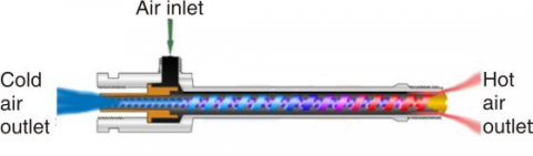
As shown schematically in Figure 1, vortex tubes can create two air streams including hot and cold using an ordinary supply of compressed air as a power source (with no moving parts). The compressed air is ejected tangentially through a generator into the vortex spin chamber. This air stream revolves around the vortex tube center at up to 1,000,000 RPM, then moves toward the hot end where some escapes through the control valve. The remaining air (still spinning) is forced back through the center of this outer vortex. The inner stream gives off the kinetic energy in the form of heat to the outer stream and finally exits from the vortex tube as the cold air. The outer stream exits at the opposite end as the hot air. (“2014, EXAIR.com”)[1].
Figure 1. Schematic drawing of a vortex tube
The vortex tube was invented accidentally in 1933. Ranque [2], a French physics student, saw the energy separation process for the first time, when he was experimenting with a vortex-type pump. He noticed that the warm air exits from one end, and cold air from the other. Ranque soon forgot his pump and started a small firm to exploit the commercial potential regarding this strange device that produced hot and cold air with no moving parts. However, it soon failed and the vortex tube slipped into obscurity until 1947 when Rudolph Hilsch [3], a German physicist, published a widely read scientific paper on the device. Other investigators have attributed the process of energy separation to the work transfer via some compression and expansion procedures. Several definitions regarding this theory are described in the literature. Harnett and Eckert [4] studied on the turbulent eddies and Ahlborn and Gordon [5] described an embedded secondary circulation. Stephan et al. [6] proposed the formation of Gortler vortices on the inside wall of the vortex tube that drive the fluid motion. Kurosaka [7] reported the temperature separation to be a result of acoustic streaming effect that transfers energy from the cold core to the hot outer annulus. Gutsol [8] assumed that the energy separation can be a consequence of the interaction between the micro volumes in the vortex tube. Despite all the proposed theories, none of them has been able to explain the temperature separation effect satisfactorily. Recent efforts have successfully utilized the computational fluid dynamics (CFD) models to explain the fundamental principles behind the energy separation produced by the vortex tube. Frohlingsdorf et al. [9] modeled the flow within a vortex tube using a CFD solver that included compressible and turbulence effects. The numerical predictions qualitatively predicted the experimental results presented by Bruun [10]. Aljuwayhel et al. [11] employed a computational fluid dynamics model to understand the process that drives the temperature separation phenomena in a vortex tube. They reported that the energy separation is due to the work transfer caused by a torque produced by viscous shear acting on a rotating control surface that separates the cold and the hot flow regions. Skye et al. [12] used a model similar to that of Aljuwayhel et al. [11]. They measured the inlet and the outlet temperatures of the flows to present a comparison analysis between the predictions from the fluid dynamics model and the experimental results. Bramo and Pourmahmoud [13] studied numerically the effect of length to diameter ratio (L/D) on the vortex tube performance and the importance of the stagnation point situation in flow patterns. In vortex tube, shape type and number of inlet nozzles are very important. So far, many investigations have been implemented on these parameters to achieve the best performance of vortex tube based on the minimum cold outlet temperature. Kirmaci and Uluer [14] investigated the vortex tube performance experimentally. They used some chambers with 2, 3, 4, 5 and 6 nozzles applying the inlet pressures varying from 150 KPa to 700 KPa, and the cold mass fractions of 0.5–0.7 (air as the working fluid). Prabakaran and Vaidyanathan [15] investigated the effect of nozzle diameter on the energy separation process. Shamsoddini and Hossein Nezhad [16] numerically investigated the effects of nozzles number on the flow and the cooling power of a counter flow vortex tube. They concluded that as the number of nozzles is increased, the cooling power increases significantly, while the cold outlet temperature decreases moderately. Rafiee and Rahimi [17] investigated the energy separation enhancement in a vortex tube using convergent nozzles experimentally and numerically, simultaneously. They studied the effect of the convergence ratio of nozzle in the range of 1-2.85. Behera et al. [18] studied the effect of shape and number of nozzles, numerically. All of mentioned investigations reported that the shape of inlet nozzles should be designed such that the flow enters tangentially into the vortex chamber. Pourmahmoud et al. [19, 20] numerically investigated the effect of helical nozzles on the performance and the cooling capacity of a vortex tube. They also introduced a new parameter named GPL (nozzle inlet gap per length of nozzle) to design this kind of nozzles. Pourmahmoud et al. [21] investigated secondary vortex chamber effect on the cooling capacity enhancement of vortex tube. Also Pourmahmoud et al. [22] investigated numerically the inlet pressure effects on the energy separation in a vortex tube with convergent nozzles and one vortex chamber. Lorenzini and Spiga [23] studied the flow field inside vortex tube. They derived some relations for the velocity components inside the vortex tube. Pourmahmoud et al. [24] studied the effect of convergent nozzles on the energy separation in a vortex tube. Pourmahmoud et al. [25] numerically investigated the effect of vortex tube length as a designing criterion.
2.1. Vortex tube model description
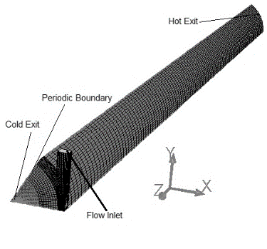
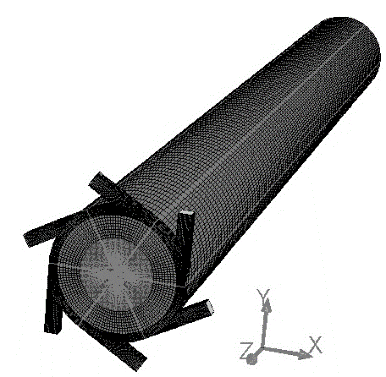
In this study, the Skye’s standard model is applied with conservation of all initial conditions. The vortex tube wall is divided into 21 equal parts, so that it contains 21 surface elements, as shown in Fig. 2. The vortex tube geometrical parameters are proposed in Table 1. Skye’s model is a vortex tube with six straight nozzles. Since, the geometry of the vortex tube can be assumed as a periodic domain, only a sector of this domain is taken for computational process. This model has been latticed regularly with 131712 cell volumes. Each of the surface elements can get different boundary condition from its adjacent elements. The mentioned boundary conditions were defined and the operation of vortex tube was investigated applying FLUENT 6.3.26.
(a)
(b)
(c)
Figure 2. (a) 3-D model of Skye’s vortex tube, (b) a sector of computational domain, (c) the wall divided into 21elements
Table 1. Geometric summery of CFD models used for vortex tube
|
Measurement |
Skye et al. (2006) experimental vortex tube |
|
Working tube length |
106 mm |
|
Working tube I.D. |
11.4 mm |
|
Nozzle height |
0.97 mm |
|
Nozzle width |
1.41 mm |
|
Nozzle total inlet area(An) |
8.2 mm2 |
|
Cold exit diameter |
6.2 mm |
|
Hot exit area |
95 mm2 |
|
Side area of vortex tube |
3.8e-3m2 |
|
Side area of an element |
1.8e-4m2 |
2.2. Boundary condition
The boundary conditions are considered based on the experimental measurements by Skye et al. (2006) [12]. The inlet is modeled as the mass flow inlet boundary condition and the vector directions are specified. The specified total mass flow rate and the stagnation temperature (at injectors) are fixed at 8.35 gr.s-1 and 294.2 K, respectively. The air flow is considered as an ideal, fully turbulent and compressible gas flow. The static pressure at the cold exit boundary was fixed at the experimental measurements (0.15 bar absolute). The static pressure at the hot exit boundary is adjusted in the way to vary the cold mass fraction. Since the CFD model predicts that the reversed flows will occur at the cold exit (at low cold gas fractions), so the backflow temperature value is set as 290 K. The boundary conditions are kept same for all models during the analysis. The tube walls are considered as adiabatic surfaces with no slip conditions. In the present research, since the flow field inside the vortex tube is assumed as a periodic domain, only a part of complete model is taken to be simulated.
2.3. Validation
In the present computations, a compressible form of the Navier-Stokes equations has been solved numerically using the FLUENTTM software package together with the k-ε turbulence model. One important parameter which indicates the vortex tube performance and the temperature separation is cold mass fraction (α) that can be defined as the ratio of the air exiting through the cold end to the pressurized inlet air. This parameter can be calculated using Eq. (1). The cold mass fraction can be controlled by a conical valve, which is placed at the hot end of the tube.
$\alpha=\frac{\dot{m}_{c}}{\dot{m}_{i n}}$(1)
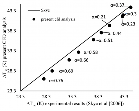
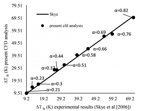
As illustrated in Figures 3 and 4, the obtained cold and hot exit temperature differences (for a vortex tube with 6 straight nozzles) were compared with the experimental results presented by Skye et al. (2006) [12]. Both models were created based on similar geometries and boundary conditions. As seen in figures, the results of the present CFD analysis are very close to the experimental results. As shown in Figure. 3, the maximum ∆Tc is obtained at the cold mass fraction (α) of 0.3 through the experimental setup and the CFD simulation. The applied 3D CFD model can produce the hot gas temperature of 363.2 K at α =0.8 and the minimum cold gas temperature of 250.24 K at 0.3 cold mass fraction.
Figure 3. Comparison of cold exit temperature difference with the experimental data at Pin=4.8(bar) and different cold mass fractions
Figure 4. Comparison of hot exit temperature difference with the experimental data at Pin=4.8(bar) and different cold mass fractions
Using shell heat transfer creates some great temperature gradients near the walls which lead to produce two vortex mixings; also these gradients increase the separation effect.
This paper focuses on an astute investigation on the effects of the mentioned temperature gradients near the walls, also tries to analyze the variation of governing equations in the system (especially the energy equation).
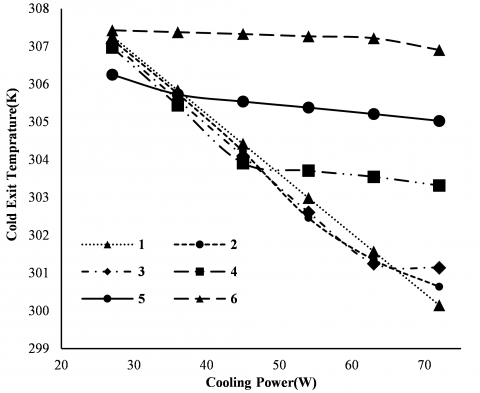
The netted vortex was considered under some negative heat fluxes and each element was cooled under various powers in the range of 27W to 72W. As seen in Figure5, an increase in the cooling power (regarding the first element which is near the nozzles) leads to severe and nonlinear changes in the temperature of cold exit. As the elements gets away from the vortex chamber, the effect of cooling power increment on the cold exit temperature decreases.
Indeed, from element 2 to element 5, the cold exit temperature changes slowly reduced by increasing cooling power. Finally, in the case of the 6th element, when the cooling power increases, the cold exit temperature remains constant. This condition is also established for the following elements. Therefore, elements 1 to 5, called the effective cooling zone as determined in Figure 7.
Figure 5. Cold exit temperature versus cooling power for each element from 1 to 6(effective cooling zone)
The cooling effects on the cold exit temperature diminishes with moving along the working tube from the vortex chamber toward the the control valve place.
Figure 6. Hot exit temperature versus cooling power for each element from 1 to 6 (effective cooling zone)
This paper tries to use the highest thermal power in order to achieve the maximum effective cooling area. This area includes 5 first elements which includes approximately 23% of the vortex tube length.
Figure 7. Effective cooling zone in the vortex tube
With respect to the mentioned statements, it could be understand that the temperatures of cold and hot exits can be affected simultaneously.
For more investigation along the whole length of vortex tube, the cooling power of 36 w was applied to all of elements. In this case, the cold exit temperature was defined for each element.
Figure 8. Cold exit temperature changes with applying the cooling power of 36 w for each element (from element 1 to 21)
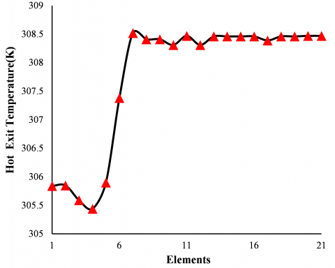
As shown in Figure 8, the significant changes cannot be seen in the cold exit temperature regarding each element after the fifth element. Also, the hot exit temperature (severely) changes up to seventh element, then remains around a constant value as observed in Figure 9.
The cold and hot exits have different thermal changing patterns in the effective cooling zone. In addition, in the effective cooling zone, the cold exit temperature strictly increases, but the hot exit temperature, first decreases and then extremely increases.
Table 2. Different cooling powers employed in system
|
heat flux ( $w / m^{2}$ ) |
heat power (w) |
|
25000 |
22.5 |
|
50000 |
45 |
|
100000 |
90 |
|
112222 |
101 |
|
150000 |
135 |
|
200000 |
180 |
Figure 9. Hot exit temperature changes with applying the cooling power of 36 w for each element (from element 1 to 21)
Effective cooling zone is considered as an operational area. The study of vortex tubes can be made with respect to the changes in the flow patterns and accordingly changes in the velocity and the pressure fields. The determination of the maximum thermal power generated by the system (set it as the base of investigations) is very important to start the cooling operation. Based on thermodynamic investigation of the vortex tube (Skye’s model), it can be observed that the maximum generated thermal power exits from the hot outlet. So, for the cooling, it is required to use the thermal power over than thermal power generated by the vortex tube. According to the following calculations, the generated thermal power by vortex tube is 101 w.
inlet airtemperature=294.2 k
hot exit temprature $=311 \mathrm{k}$
Cold exit temperature = 250 k
$\dot{m}_{i}=8.35^{g r} /_{S^{*}}$
$\alpha=\frac{\dot{m}_{c}}{\dot{m}_{i}}=0.298$
$c_{p} )_{a i r}=1006^{j} /_{k g . k}$
$\dot{Q}_{h}=\dot{m}_{h} c_{p}\left(T_{h}-T_{i}\right)=101 \mathrm{w}$(2)
$\dot{Q}_{c}=\dot{m}_{c} c_{p}\left(T_{i}-T_{c}\right)=105 \mathrm{w}$(3)
The cooling operation is performed in the effective cooling zone (Table 2) considering the amount of thermal power generated.
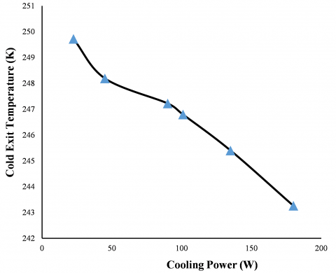
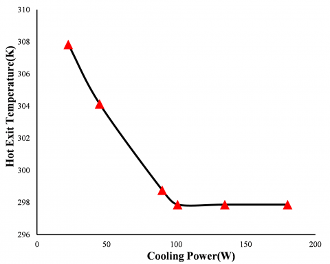
Figure 10.The effect of cooling power (applied to effective cooling zone) on cold exit temperature
As seen in Figure 10, the temperature of cold exit decreases with increase in the cooling power. Also, the temperature of hot exit decreases up to a certain amount (298 k) with enhancing the cooling power, but after 90 w, the cooling power increment cannot effect on the temperature of hot outlet, so, it remains constant. As illustrated in Figure11.
Figure 11. Behavior of the hot exit temperature with various cooling powers applied to the effective cooling zone
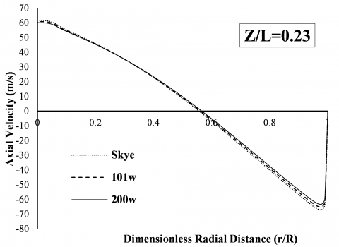
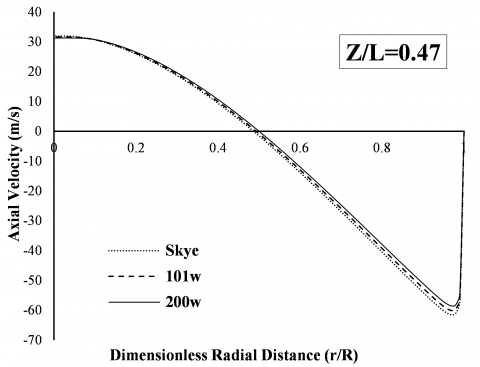
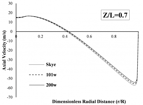
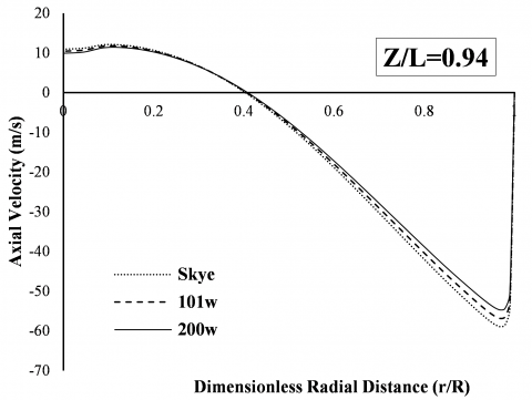
To make these changes (caused by cooling on the flow pattern) visible, it is necessary to investigate the flow pattern difference between the Skye’s and the present models. As a comparison example, 101, 200 cooling powers are applied to clarify the differences between the flow patterns inside the vortex tube. Therefore, the axial velocity is studied first. As seen in Figure12. The axial velocity diagram is drawn for 4 states. Axial velocity is declined gradually at the center of vortex tube with increasing cooling power. Also, the maximum axial velocity occurs at 101 w in all cases. The reduction of axial velocity inside the vortex tube is due to the cooling flux on the wall, which affects the boundary layer around the wall and is an obstacle to increase the axial velocity.
(a)
(b)
(c)
(d)
Figure 12. Axial velocity profiles in 4 different dimensionless longitudinal distances (z/l=0.23, z/l=0.47, z/l=0.7, z/l=0.94)
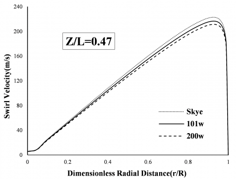
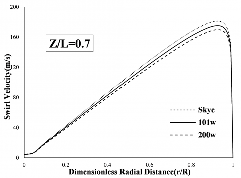
There are also changes in the swirl velocity, whatever the cooling power rate increases the swirl velocity decreases. As seen in Figure 13, the swirl velocity profiles are shown for different sections. The maximum difference in swirl velocity is 80% at radial distance of 0.94.
(a)
(b)
(c)
(d)
Figure 13. Swirl velocity profiles in 4 various dimensionless longitudinal distances (z/l=.23, z/l=.47, z/l=.7, z/l=.94)
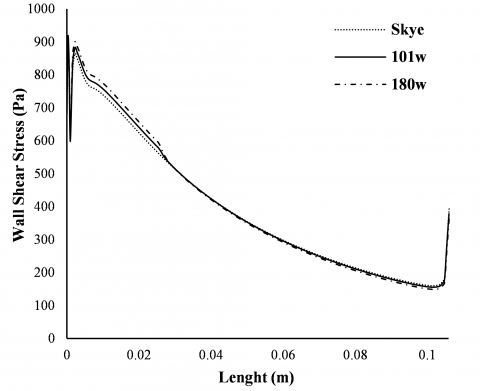
Shear stress on the wall also is investigated for different modes of cooling. According to the amount of selected cooling power, the shear stress at the effective cooling zone is affected and increased. As the air passes through the effective cooling zone, its pressure is dropped and shear stress is reduced on the wall. As seen in Fig 14, the shear stress value is lower than that of the Skye’s model (at the hot end of the vortex tube).
Figure 14. Wall shear stress along the length of vortex tube (in 4 different cooling powers)
The reasons of why the cooling effect on the temperature of both hot and cold outlets (simultaneously) is just at the beginning of vortex tube can be explained as: first, the axial velocity at the beginning of the vortex tube is lower compared to other areas, so, the air has a chance to exchange the heat, second, temperature reduction in primary vortex causes a decrease in disturbances between the layers, on the other side, decreasing volume of the hot vortex and increasing expansion of interior vortex will follow further temperature reduction.
The use of shell heat transfer mechanism has been proposed as a new approach to change the flow pattern in the vortex tube. According to the performed analysis the following topics can be picked up: in order to find the best zone for affecting the temperature of cold end, the Skye’s model has been divided into equal elements and all the elements have been placed under heat flux according to the selected reference in the vortex tube. Considering the different amounts of negative heat flux on the wall of the vortex tube, just 5 first elements were introduced as the effective cooling zone. Outside the effective cooling zone, there is no change in the temperature of the cold outlet for every cooling power (almost). Also, the temperature is reduced to the certain temperature at the hot end. Because, the axial velocity is so large for outside of the effective cooling zone, therefore, the air has limited opportunities to get influence. In the case of effective cooling zone, the increasing cooling power in addition to reduce the temperature of hot end to a certain temperature, can help the temperature of cold end to change in any extent. The cooling power of 101 W was selected as the reference power .This amount is equivalent to the wasted heat from the hot end of the Skye’s model.
Heat transfer from the vortex tube creates major temperature gradients near the wall, which cause the changes in the speed of initial vortex. As a result, the heat transfer reduces the effects of separation in the first but along the vortex tube due to the temperature drop of air, the effect of separation is optimized and the temperature is reduced at the cold end.
Generally, it should be said that any changes in the boundary conditions of the vortex tube wall in the effective zone, leads to reduction in the air rotational speed. In other words, the current pattern will result different flow pattern from Skye’s model. The reason is that the new boundary condition increases the shear stress and operates as a hedge against the air moving.
|
D |
Diameter of vortex tube (mm) |
|||
|
k |
Turbulence kinetic energy (m2/s2) |
|||
|
L |
Length of vortex tube (mm) |
|||
|
r |
Radial distance measured from centerline of tube (mm) |
|||
|
R |
Radius of vortex tube (mm) |
|||
|
T |
Temperature (K) |
|||
|
z |
Axial length from nozzle cross section (mm) |
|||
|
$\Delta \mathrm{T}_{\mathrm{i}, \mathrm{c}}$ |
Temperature difference between inlet and cold end (K) |
|||
|
$\Delta \mathrm{T}_{\mathrm{i}, \mathrm{h}}$ |
Temperature difference between inlet and hot end (K) |
|||
|
$\dot{\mathrm{m}}_{\mathrm{in}}$ |
Inlet mass flow rate (kg/s) |
|||
|
$\dot{\mathrm{m}}_{\mathrm{c}}$ |
Cold mass flow rate (kg/s) |
|||
|
$\dot{\mathrm{m}}_{\mathrm{h}}$ |
Hot mass flow rate (kg/s) |
|||
|
Greek symbols |
||||
|
$\alpha$ |
Cold mass fraction |
|||
|
$\varepsilon$ |
Turbulence dissipation rate (m2/s3) |
|||
|
$\rho$ |
Density (kg/m3) |
|||
|
$\mu$ |
Dynamic viscosity (kg/(m s)) |
|||
|
$\mu_{t}$ |
Turbulent viscosity (kg/(m s)) |
|||
|
$\tau_{\mathrm{ij}}$ |
Stress tensor components |
|||
|
Subscripts |
||||
|
h |
hot |
|||
|
i |
inlet |
|||
|
c |
cold |
|||
APPENDIX
Governing equations
The numerical modeling of the vortex tube has been carried out with the Fluent Code (version: 6.3.26). This computer program allows calculations for compressible fully turbulent flows. The governing equations per unit volume can be solved by Fluent for general fluid flows. These equations can be given as follows:
$\frac{\partial}{\partial x_{j}}\left(\rho u_{j}\right)=0$(A.1)
$\frac{\partial}{\partial x_{j}}\left(\rho u_{i} u_{j}\right)=-\frac{\partial p}{\partial x_{i}}+$
$\frac{\partial}{\partial x_{j}}\left[\mu_{e f f}\left(\frac{\partial u_{i}}{\partial x_{j}}+\frac{\partial u_{j}}{\partial x_{i}}-\frac{2}{3} \delta_{i j} \frac{\partial u_{k}}{\partial x_{k}}\right)\right]+\frac{\partial}{\partial x_{j}}\left(-\overline{\rho} \overline{u}_{i}^{\prime} \overline{u}_{j}^{\prime}\right)$
$\mu_{e f f}=\mu+\mu_{t}$(A.2)
$\frac{\partial}{\partial x_{i}}\left[u_{i} \rho\left(h+\frac{1}{2} u j u_{j}\right)\right]=\frac{\partial}{\partial x_{j}}\left[k e f f \frac{\partial T}{\partial x_{j}}+u_{i}\left(\tau_{i j}\right)_{e f f}\right]$
$k_{e f f}=K+\frac{c p^{\mu} t}{\operatorname{Pr} t}$(A.3)
The previous equations are continuity, momentums and energy, respectively. Since we assumed the working fluid as an ideal gas, so, the compressibility effect must be imposed so that:
$p=\rho R T$(A.4)
$\frac{\partial}{\partial t}(\rho k)+\frac{\partial}{\partial x_{i}}\left(\rho k u_{i}\right)=\frac{\partial}{\partial x_{j}}\left[\left(\mu+\frac{\mu_{t}}{\sigma_{k}}\right) \frac{\partial k}{\partial x_{j}}\right]$$+G k^{+} G b^{-} \rho \varepsilon-Y M$(A.5)
$\frac{\partial}{\partial t}(\rho \varepsilon)+\frac{\partial}{\partial x_{i}}\left(\rho \varepsilon_{u_{i}}\right)=\frac{\partial}{\partial x_{j}}\left[\left(\mu+\frac{\mu_{t}}{\sigma_{\mathcal{E}}}\right) \frac{\partial \varepsilon}{\partial x_{j}}\right]+$$C_{1 \varepsilon} \frac{\varepsilon}{k}\left(G_{k}+C_{3 \varepsilon} G_{b}\right)-C_{2 \varepsilon} \rho \frac{\varepsilon^{2}}{k}$(A.6)
Flow in the vortex tube is highly turbulent. The steady state assumption and practical considerations indicate that a turbulence model must be employed to represent its effects. The standard k-ε turbulence model is applied to the compressible Navier-Stokes equations for numerical analyzing of computational domain. The turbulence kinetic energy, k, and its rate of dissipation, $\boldsymbol{\varepsilon}$ are obtained from the following transport equations: In these equations, $\mathrm{G}_{\mathrm{k}}$ represents the generation of turbulence kinetic energy due to the mean velocity gradients, $\mathrm{G}_{\mathrm{b}}$ is the generation of turbulence kinetic energy due to buoyancy that is neglected. $\mathrm{Y}_{\mathrm{M}}$ Indicates the contribution of the fluctuating dilatation in compressible turbulence to the overall dissipation rate, and finally$\mathrm{C}_{1 \varepsilon}, \mathrm{C}_{2 \varepsilon},$ and $\mathrm{C}_{3 \varepsilon}$ are constants values. These default values have been determined from experiments with air and water for fundamental turbulent shear flows including homogeneous shear flows and decaying isotropic grid turbulence. $\sigma_{\varepsilon}$ and $\sigma_{\mathrm{k}}$ are the turbulent Prandtl numbers for k and $\mathcal{E}$,respectively. The turbulent (or eddy) viscosity,$\mu_{\mathrm{t}}$ is computed by combining k and $\varepsilon$ as follows:
$\mu_{t}=\rho C_{\mu} \frac{k^{2}}{\varepsilon}$(A.7)
where, $C_{\mu}$ is a constant. The model constants C1ε, C2ε, Cμ, σk and σε have the following default values: C1ε = 1.44, C2ε = 1.92, Cμ = 0.09, σk = 1.0, σε = 1.3. Finite volume method with a three-dimensional mesh is used and the boundary conditions are applied. Air is used as an ideal gas and the flow is assumed compressible. Second Order Upwind scheme is used to discretize convective terms, and SIMPLE procedure is used to solve the momentum and energy equations simultaneously. The cold exit temperature difference (ΔTc) and the hot exit temperature difference (ΔTh) of the vortex tube are defined as following, respectively:
$\Delta \mathrm{T}_{\mathrm{c}}=\mathrm{T}_{i}-\mathrm{T}_{\mathrm{c}}$(A.8)
$\Delta \mathrm{T}_{\mathrm{h}}=\mathrm{T}_{\mathrm{h}}-\mathrm{T}_{i}$(4.9)
Cold mass fraction is the percentage of the air exits through the cold end of the vortex tube to the pressurized air input and can be calculated by using Eq. (10).
[1] Vortex Tube & Spot Cooling Products, Exair Corporation, http://www.exair.com.
[2] G. J. Ranque, “Experiments on expansion in a vortex with simultaneous exhaust of hot air and cold air,” J. Phys. Radium (Paris), vol. 4, pp. 112-115, 1933.
[3] R. Hilsch, “The use of the expansion of gases in a centrifugal field as cooling process,” Rev Sci Instrum, vol. 18, pp. 108-113, 1947. DOI: 10.1063/1.1740893.
[4] J. Harnett and E. Eckert, “Experimental study of the velocity and temperature distribution in a high velocity vortex-type flow,” Transcation of ASME, vol. 79, pp. 751-758, 1957.
[5] B. K. Ahlborn and J. M. Gordon, “The vortex tube as a classic thermodynamic refrigeration cycle,” Journal of Applied Physics, vol. 88 no. 6, pp. 3645-3653, 2000. DOI: 10.1063/1.1289524.
[6] K. Stephan, S. Lin, M. Durst, F. Huang, and D. Seher, “An investigation of energy separation in a vortex tube,” International Journal of Heat and Mass Transfer, vol. 26 no. 3, pp. 341–348, 1983. DOI: 10.1016/0017-9310(83)90038-8.
[7] M. Kurosaka, “Acoustic streaming in swirling flows,” Journa of Fluid Mechanics, vol. 124, pp. 139–172, 1982. DOI: 10.1017/S0022112082002444.
[8] A. F. Gutsol, “The Ranque effect,” Physics Usp, vol. 40, pp. 639–658, 1997. DOI: 10.1070/PU1997v040n06ABEH000248.
[9] W. Frohlingsdorf and H. Unger, “Numerical investigations of the compressible flow and the energy separation in the Ranque–Hilsch vortex tube,” International Journal of Heat and Mass Transfer, vol. 42, pp. 415–422, 1999. DOI: 10.1016/S0017-9310(98)00191-4.
[10] H. H. Bruun, “Experimental investigation of the energy separation in vortex tubes,” Journal of Mechanical Engineering Science, vol. 11, pp. 567-582, 1969. DOI: 10.1243/JMES_JOUR1969_011_070_02.
[11] N. F. Aljuwayhel, G. F. Nellis and S. A. Klein, “Parametric and internal study of the vortex tube using a CFD model,” International Journal of Refrigeration, vol. 28, pp. 442–450, 2005. DOI: 10.1016/j.ijrefrig.2004.04.004.
[12] H. M. Skye, G. F. Nellis and S. A. Klein, “Comparison of CFD analysis to empirical data in a commercial vortex tube,” International Journal of Refrigeration, vol. 29, pp. 71–80, 2006. DOI: 10.1016/j.ijrefrig.2005.05.004.
[13] A. R. Bramo and N. Pourmahmoud, “Computational fluid dynamics simulation of length to diameter ratio effect on the energy separation in a vortex tube,” Thermal Science, vol. 15, no. 3, pp. 833–848, 2011.
[14] V. Kirmaci and O. Uluer, “An experimental investigation of the cold mass fraction, nozzle number and inlet pressure effects on performance of counter flow vortex tube,” Journal of Heat Transfer-Transactions. ASME, vol. 8, no. 131, pp. 081701–081709, 2009.
[15] J. Prabakaran and S. Vaidyanathan, “Effect of diameter of orifice and nozzle on the performance of counter flow vortex tube,” International Journal of Engineering Science and Technology, vol. 2 no. 4, pp. 704-707, 2010.
[16] R. Shamsoddini and A. HosseinNezhad, “Numerical analysis of the effects of nozzles number on the flow and power of cooling of a vortex tube,” International of Journal Refrigeration, vol. 33, pp. 774–782, 2010. DOI: 10.1016/j.ijrefrig.2009.12.029.
[17] S. E. Rafiee and M. Rahimi, “Experimental study and three-dimensional (3D) computational fluid dynamics (CFD) analysis on the effect of the convergence ratio, pressure inlet and number of nozzle intake on vortex tube performance-validation and CFD optimization,” Energy, vol. 63, pp. 195-204, 2013. DOI: 10.1016/j.energy.2013.09.060.
[18] U. Behera and P. J. Paul, S. Kasthurirengen, R. Karunanithi, S. N. Ram, K. Dinesh and S. Jacob, “CFD analysis and experimental investigations towards optimizing the parameters of Ranque–Hilsch vortex tube,” International Journal of Heat and Mass Transfer, vol. 48, pp. 1961–1973, 2005. DOI: 10.1016/j.ijheatmasstransfer.2004.12.046.
[19] N. Pourmahmoud, A. Hassanzadeh, O. Moutaby and A. R. Bramo, “Computational fluid dynamics analysis of helical nozzles effects on the energy separation in a vortex tube,” Thermal Science, vol. 16, no. 1, pp. 149–164, 2012a.
[20] N. Pourmahmoud, A. Hassanzadeh and O. Moutaby, “Numerical analysis of the effect of helical nozzles gap on the cooling capacity of Ranque–Hilsch vortex tube,” International Journal of Refrigeration, vol. 35, no. 5, pp. 1473-1483, 2012b. DOI: 10.1016/j.ijrefrig.2012.03.019.
[21] N. Pourmahmoud, F. Sepehrian Azar and A. Hassanzadeh, “Numerical simulation of secondary vortex chamber effect on the cooling capacity enhancement of vortex tube,” Heat Mass Transfer, vol. 50, pp. 1225–1236, 2014a. DOI: 10.1007/s00231-014-1335-z.
[22] N. Pourmahmoud, M. Rashidzadeh and A. Hassanzadeh, “CFD investigation of inlet pressure effects on the energy separation in a vortex tube with convergent nozzles,” Engineering Computations, vol. 32 no. 5, 2015, pp. 1323-1342, 2014b. DOI: 10.1108/EC-06-2014-0125.
[23] E. Lorenzini and M. Spiga, “Fluid dynamic isotopic separation by the Hilsch vortex tube,” (in Italian), Ingegneria, no. 5-6, pp. 121-126, Maggio-Giugno, 1982.
[24] N. Pourmahmoud, A. Hassanzadeh, E. Rafiee and M. Rahimi, “Three-Dimensional numerical investigation of effect of convergent nozzles on the energy separation in a vortex tube,” Int. J. Heat Tech., vol. 30, no. 2, pp. 133-140, 2012. DOI: 10.18280/ijht.300219.
[25] N. Pourmahmoud, R. Esmaily amd A. Hassanzadeh, “CFD investigation of vortex tube length effect as a designing criterion,” Int. J. Heat Tech., vol. 33, no.1, 2015. DOI: 10.18280/ijht.330118.