OPEN ACCESS
In this work, a pipe provided with twisted tape inserts is analyzed. This system allows a significant increase of convective heat transfer coefficient by introducing a swirl motion which determines greater heat removal from the solid surface, by improving the fluid mixing. The analysis performed in this paper focuses on the evaluation of the thermal and flow quantities for a pipe of a shell and tube heat exchanger, previously optimized through a design software widely used in the petrochemical industry. The thermo and fluid dynamics analysis were performed by using a commercial CFD software (FluentTM). After performing the necessary computational checks for the acceptance of the results provided by the solver, a pitch parameterization was performed through a finite volume simulation. In this way the behaviour of a highly viscous fluid was studied, whose thermo-physical characteristics are highly variable with temperature. Furthermore, using water as fluid, the behaviour of the pipe provided with inserts was investigated by varying the Reynolds number, through mass flow rate variation. To verify the correctness of the results, they were compared in both cases with correlations in the literature.
Heat, Exchange, Twisted, Tape pipe, CFD, Analysis.
In the petrochemical industry great attention is paid to the optimization of heat exchangers during the design phase, to minimize the overall dimensions of the equipment. When the heat exchange process is not very efficient, mechanical inserts are often used. They increase the efficiency of heat exchange operating upon the boundary layer by introducing a swirl motion and increasing the mixing of the fluid from the wall towards the bulk. In this way an increase in the convective heat transfer coefficient is obtained, while the size of the equipment decreases.
In this paper, the thermo and fluid dynamic properties of a flow within a pipe, provided with twisted tape inserts, were analyzed through CFD numerical analysis by using the finite volume method. In this study the pipe wall was considered to have a constant heat flux and the turbulator was considered adiabatic. Moreover, in the CFD software the conditions of “mass flow inlet” and “outflow” were used. The simulations were performed by solving the Navier-Stokes equations.
A first analysis was conducted for a pipe with a length of 500 mm. For this configuration crude oil was used, as is usual in the petrochemical industry. The complete development of the hydrodynamic boundary layer was also verified. The high viscosity of the fluid, together with the low inlet velocity in the pipe, implies a very low value of the Reynolds number. It indicates a full laminar flow.
The insertion of this type of turbulator introduces a swirl motion, which increases the kinetic energy of the flow that means it can be defined as pseudo-laminar, as confirmed by Sarma et al. [1]. The resolution of the flow field, for low Reynolds numbers, through a two-equations turbulence model (k-ω), provides the same results obtained by using the laminar model.
Different twist ratio resolutions were compared for the same geometry. Also, in order to make a comparison, CFD analysis was applied to a pipe with a length of 8,000 mm. It is part of a real heat exchanger dimensioned and optimized by using HTRI software [2], widely used by petrochemical companies.
In order to evaluate the mean value of the convective heat transfer coefficient by varying the Reynolds number, the last analysis concerned a pipe with a length of 1,500 mm using water as the working fluid. CFD simulations results were finally compared with those obtained by the application of some correlations available in the literature [3], [4].
Heat exchangers have multiple applications. Their design is complex and requires an accurate analysis to estimate the thermal power and pressure losses. Their design also requires an estimate of the performances in the long term and an accurate economic analysis.
The exchange surface or the convective heat transfer coefficient can be changed to increase the thermal power. Introducing, for example, a “disorder” in the fluid motion a discontinuity in the velocity and temperature boundary layer could be generated. It results in a reduction of their thickness. The disorder can be obtained by using mechanical inserts which improve the heat exchange and thermal efficiency. The choice of the material of the turbulators is suggested by the aggressiveness of the fluid with which they are in contact. In general they are made of the same material as the pipes in which they are inserted [5].
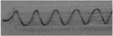
Figure 1. Helical Wire Coil insert
Figure 2. hiTRAN wire matrix element, Courtesy of Cal Gavin LTD, UK [11]
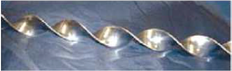
Figure 3. Twisted tape insert
The experimental studies conducted to check the thermal and hydraulic performance of these devices have shown that they lead to an improvement of the performance of heat exchangers, with an increase in pressure losses, caused by the same mechanisms that lead to the improvement of the thermal exchange.
The most common types of turbulator are: Helical Wire Coil (Figure 1), consisting of a metal wire wrapped like a helix; Wire Mesh (Figure 2), consisting of metal wires twisted to form a core on which a metal matrix is formed; Twisted tape (Figure 3), consisting of a twisted metal baffle. The latter is analyzed in the present work.
2.1 Twisted tape
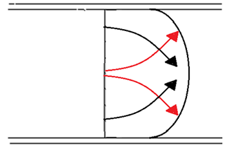
Twisted tapes are inserts of predefined size, to which a torque is applied to impart the characteristic helical shape. The flow is fundamentally altered because the turbulator impresses a swirl motion that causes an increase in flow path. An increase in the axial velocity owing to the reduction of the hydraulic diameter, the generation of secondary motion components which improve the mixing between the fluid in correspondence of the bulk and the wall, allow the boundary layers to be modified by increasing the velocity and temperature gradients (Figure 4). In this way, the resistance to heat exchange and the difference between the wall and the bulk temperature are reduced, increasing the heat transfer coefficient on the wall [6].
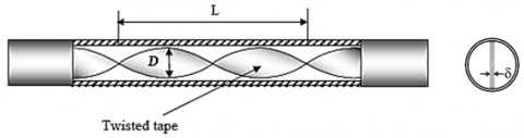
The geometric characteristics, in Figure 5, are represented by the thickness of the tape δ, its width D nearly coincident with the size of the pipe diameter, with the exception of a very small gap of a few millimetres, and the twist ratio L/D. In addition to the reasons already mentioned, the easy manufacturing and assembling dictate the convenience in the use of twisted tape.
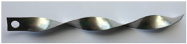
Figure 6 shows a sample of the twisted tape prototype. In the initial part of the twisted tape there is a hole that is used to insert a plug that will block the twisted tape in the pipe. The twisted tape can be easily pulled out of the pipe and again reinserted to facilitate maintenance operations [5].
Figure 4. Mechanism of mixing with use of twisted tape turbulator
Figure 5. Representation of a twisted tape inside a pipe
Figure 6. Prototype of twisted tape
The increase in the convective heat transfer coefficient owing to the use of twisted tapes causes the superimposition of five effects [1]. These effects are: the increase in velocity due to the partitioning of the flow, the reduction of the hydraulic diameter, the increase of the flow path due to the presence of the tape, the generation of a secondary flow due to the spin induced by insert and, in the case of good contact between the insert and wall pipe, the fin effect.
The major influence on the increase of convective heat transfer coefficient is due to the strong mixing of the fluid for the occurrence of a centrifugal motion. This generates a vortex inside the flow and produces a tangential velocity component, negligible in the case of one-dimensional flow typical of a pipe without insert, with the consequent increase in the velocity modulus.
In the case of a completely laminar flow, with Re<2,300, the generation of a swirl motion determines the presence of a turbulence. The flow corresponding to this particular flow field is defined as pseudo-laminar [1].
Because of the complexity of the flow and temperature field it is necessary to use advanced numerical tools for the study of the problem. In the present work Fluent was used solving the problem with the finite volume method.
3.1 Data and geometry of the problem
The main incognitos of the problem is the convective heat transfer coefficient h. In order to determine the variation of heat transfer coefficient as a function of the twist ratio and mass flow rate a parametric study was performed.
Because of the large number of simulations, the study of the twisted tape, by varying the twist ratio, was applied to a pipe with a length of 500 mm that corresponds to about 30 times the internal diameter. For this configuration the full development of the hydrodynamic boundary layer is verified but this is not true for the thermal boundary layer.
Table 1 shows the geometric characteristics of the pipe and insert used for the simulations.
Table 1. Geometric characteristics of the pipe and of the turbulator
|
External diameter of the pipe $\varphi_{e x t}$[mm] |
19.05 |
|
|
Thickness of the pipe s [mm] |
1.651 |
|
|
Pipe length l [mm] |
500 |
|
|
Cross section of the twisted tape |
δ [mm] |
1 |
|
D [mm] |
13.5 |
|
Table 2. Thermo-physical properties of Incoloy-825
|
Density: ρinc |
8,140 |
|
Specific heat: cpinc |
440 |
|
Thermal conductivity: kinc |
11.3 |
Table 3. Thermophysical properties of crude oil
|
Density: ρco |
$\rho_{c o}=-0.7371 \cdot T+1113.5$ |
|
Viscosity: μco |
$\mu_{\mathrm{co}}=120.14 \exp (-0.025 \cdot \mathrm{T})$ |
|
Thermal conductivity: kco |
$\mathrm{k}_{\mathrm{co}}=-0.0002 \cdot \mathrm{T}+0.2082$ |
|
Specific heat: cpco |
$\mathrm{c}_{\mathrm{p} \mathrm{co}}=4.0816 \cdot \mathrm{T}+567.09$ |
Twist ratio L/D equal to 2, 4, 6, 8, 10, 12, 14, 16 and a pipe without insert were used in order to verify its influence on the convective heat transfer coefficient.
The CFD analysis was also applied to an 8-meter pipe fitted with an insert with a twist ratio of L/D = 8, in order to make comparison with some data of a real exchanger. An analysis through the use of HTRI software was also carried out [2].
3.2 Materials and fluids
The material used in all the cases studied is the Incoloy-825, both for pipe and twisted tape. It is a nickel-iron-chromium alloy with additions of molybdenum and copper. Its most important thermo-physical properties are shown in Table 2:
In simulations aimed at the study of the influence of the twist ratio, crude oil was employed as working fluid. Crude oil is a very viscous fluid whose thermo-physical characteristics vary significantly with the temperature.
For the 500 mm pipe, because of the small temperature difference between the inlet and outlet sections, the characteristics of the oil have been assumed as constants and evaluated at an average temperature between the two sections. A flow rate of oil equal to 0.041 kg/s was used.
For the 8-metre long pipe, because of the variation in the temperature of the fluid between the inlet and outlet section, its thermo-physical properties were considered as temperature dependent according to the equations reported in Table 3. In this case, a flow rate of oil equal to 0.02245 kg/s was used.
To take into account the influence of other parameters such as the Prandtl and Reynolds numbers, other simulations were carried out for the 1,500 mm pipe with a twist ratio L/D = 8. Water was used as working fluid. The convective heat transfer coefficient was evaluated by varying the Reynolds numbers in the range 500, 1000 and 1,500 which correspond to water flow rates of 9.83, 19.7 and 29.5 g/s respectively.
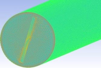
A thermo and fluid-dynamics study of the different geometries was conducted through CFD simulations. The geometry of the turbulator was generated using ICEM software, faithfully reproducing the geometric characteristics of the problem. The complexity of the geometry prevented use of a hexahedral grid because of some volume intersections near the turbulator wall. A grid of tetrahedral type was therefore chosen for both fluids, with thickening of the grid near the pipe wall (the height of the centroid of the first cell of the wall is equal to 0.075 mm). The smaller grid dimensions near the turbulator wall were performed using tetrahedral volumes.
Being a laminar flow, it was not necessary to use a particularly pushed thickening. For the gap present between the longitudinal end of the turbulator and the solid pipe wall it was necessary to use a greater number of cells in order to study the behaviour of the fluid in this area with good accuracy.
The geometry corresponding to the analysis, aimed at the study of the behaviour of the fluid in the 8-metre long pipe, did not allow the use of a large number of volumes because of the extension of the physical and computational domain. In this case the rows belonging to the boundary layer were reduced to two.
The approach by which the behaviour of the fluid in the pipe without insert was studied, was completely different. The domain generated in this case, for obvious computational reasons, is two-dimensional, axisymmetric and periodic between input and output; a square cells grid was used.
The verification of the simulation correctness was performed in reverse order, i.e. starting from the results obtained from CFD analysis and compared them with those resulting from the application of mass and energy balances.
4.1 Boundary conditions
Solid walls were modelled with the wall-type boundary condition. On the lateral surface of the pipe a constant heat flux is assigned, which determines a condition of the wall temperature variable along the axis of the pipe. In correspondence to the turbulator wall, however, an adiabatic condition was imposed because of its contact with the same temperature fluid on both faces.
Conditions of “mass flow inlet” in the input section and “outflow” at the output section were used for the fluid. The input condition is characterized by a constant mass flow rate and assigned as a function of the Reynolds number. The outflow condition allows determination of the pressure losses in the pipe by solving the continuity, momentum and energy equations.
4.2 Grid generation
The verification of the correctness of the solution obtained by the computer is performed through a backwards process, by checking the conformity between the boundary conditions and the principles of conservation:
$\mathrm{Q}_{\mathrm{in}}+\mathrm{Q}_{\mathrm{ext}}+\mathrm{Q}_{\mathrm{out}}=0$(1)
$\mathrm{Q}_{\mathrm{ext}}=\dot{\mathrm{m}} \mathrm{c}_{\mathrm{p}}\left(\mathrm{T}_{\mathrm{out}}-\mathrm{T}_{\mathrm{in}}\right)$(2)
The verification of the solution convergence, for each simulation, is considered valid when the energy balance provided by the solver gives an average temperature at the output section equal to that obtained by Eq. (2). Respect of the continuity equation was also checked.
Three computing grids named M1, M2, M3 were generated. The increase factors of the number of nodes used are equal to 1.31 between the first and second grid, 1.41 between the second and the third.
The independence of the mesh was verified on the temperature profiles considering sections respectively located at 0.0315, 0.063, 0.126, 0.315 and 0.3465 metres from the inlet section. Table 4 reports the data of the mesh independence.
The mesh independence was verified for some geometries while the others were constructed so that the number of elements was about equal to that of the mesh-independent grids. For the calculation, the root mean squared percentage error was used, as defined by Eq. (3) and it is reported in Table 4.
$R M S E P=\sqrt{\frac{\sum_{i=1}^{n}\left(\frac{x_{i}-\hat{x}_{i}}{x_{i}}\right)^{2}}{N}} \cdot 100$(3)
The interpolation of the grid points belonging to the less dense mesh was performed using an algorithm written in Matlab.
An offset value of less than 5 % was taken into account for the verification of the grid independence. It is assumed that the convergence of the iterations occurs for a stabilization of the residuals to a value of or below 10-6 for the energy equation, and 10-3 for the pressure correction equation (continuity equation). The energy and mass balances were monitored during the iterations and it was verified that they were not more than 10-17 for the mass conservation and 10-5 for the energy conservation. The grids used for the simulations performed by varying the twist ratio, were independent for a number of elements between 1.4$\cdot 10^{6}$and $1.6^{\cdot} 10^{6}$(approximately).
Figures 7 and 8 show details of the mesh used for the thermo-fluid dynamic calculation.
Table 4. Mesh independence
|
Section |
0.0315 |
0.063 |
0.126 |
0.315 |
0.3465 |
|
M1 - M2 |
0.0035% |
0.0021% |
0.0161% |
0.0660% |
0.0642% |
|
M2 - M3 |
0.0090% |
0.0018% |
0.0127% |
0.0641% |
0.0262% |
Figure 7. Mesh of the pipe provided with twisted tape
Figure 8. Mesh of the twisted tape
The results of fluid dynamics analysis, performed by varying the twist ratio of the turbulator, for the 500 mm pipe and crude oil used as working fluid, are given below. Assuming constant thermo-physical properties for the fluid, a Reynolds number of about 100 and a number of Prandtl equal to 565 are obtained.
From the hydrodynamic point of view, the motion of the fluid is completely developed at a distance of 75 mm from the inlet section.
Owing to the high value of the Prandtl number, the temperature profile is completely developed after 36 m from the inlet section. These hypotheses were verified with the correlations reported in [7], and by means of the superposition of the velocity and temperature profiles for the subsequent sections.
The study of the thermo-fluid dynamics behaviour has allowed us to evaluate the influence of the turbulator on the flow and temperature fields that are established within the pipe, the medium convective heat transfer coefficient and the performance of this as a function of the length of the pipe.
5.1 Fluid-dynamics analysis
The presence of the insert determines a partition of the flow and a slight reduction of the cross-section of the pipe; this causes a slight increase in the fluid velocity. A vortex is generated which is screwed in the axial direction and determines the occurrence of tangential velocity components which, when added vectorially to the axial component of velocity, leads to an increase in the resulting velocity vector. The magnitude of the vortex, which tends to increase with decreasing twist ratio of the turbulator, leads to a growth of the tangential component.
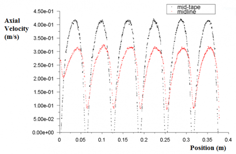
Because of the generated swirl, the trend of the velocity, in a parallel direction to the pipe axis, will not be more linear and ascending up to the completely developed condition of motion, as in the case of a pipe without insert, but it will be discontinuous and periodic because of the macro-vortex induced (Figure 9).
Figure 9. Axial velocity in the presence of the turbulator
Starting from the pipe wall, on which are shown the no-slip effects due to the interaction fluid-solid, the velocity will increase, even with not very accentuated gradient, reaching a maximum in correspondence to the central areas of the septum. These areas cannot be deemed to be in the middle of the hydraulic diameter because the effects of the tangential actions, leading to small twist ratios of the turbulator, tend to move them and to reduce the size [8]. In the limiting case of a pipe without insert, reached by twist ratios of the turbulator that tend to infinity, these areas will be positioned exactly symmetrically in relation to the inserted septum. At decrease in the twist ratio, it will tend to rotate with the embossed side toward the direction of screwing of the insert, moving in zones at the corners, as shown in Figures 10, 11 and 12.
A migration of the cores (shown in red in the figures) occurs for each value of the twist ratio, towards the edges of the turbulator, bringing the fluid to be canalized in the gap present between the solid walls. In correspondence to the gap, because of its small size (1.124 mm), important effects cannot be seen, in kinetic terms, as viscous effects prevail mainly due to the type of fluid considered (crude-oil).
Figure 10. Level curves of the axial velocity in the output section for twist ratio L/D=12
Figure 11. Level curves of the axial velocity in the output section for twist ratio L/D=8
Figure 12. Level curves of the axial velocity in the output section for twist ratio L/D=4
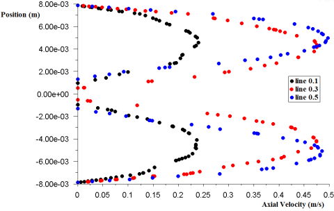
Figure 13 shows the velocity profiles as a function of axial distance, for lines placed on sections at 0.1, 0.3 and 0.5 m from the input section passing through the centre of the pipe.
Figure 14 shows, as example, the lines of flux (velocity streamline) that describe the motion field of the fluid in the presence of the insert with a twist ratio L/D = 4.
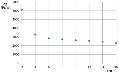
Starting from the configuration of the plain pipe, which, for simplicity, it is assumed equivalent to the case of a pipe with turbulator twist ratio tending to infinity, there is an increase in the pressure losses as the intensity of the vortex increases as a result of the reduction of twist ratio of the turbulator. The pressure losses per unit length, as shown in Figure 15, increase with twist ratio decreasing. For twist ratio of less than 6, such losses become significant causing high pumping costs. A reduction of the twist ratio from 6 to 4 causes an increase in the pressure losses of 15 %, while for a reduction from 4 to 2, the pressure losses are 88 %.
Figure 13. Trend of axial velocity (L/D=4)
Figure 14. Motion of the fluid in the presence of insert with twist ratio of L/D=4.
Figure 15. Pressure losses at varying of the twist ratio L/D
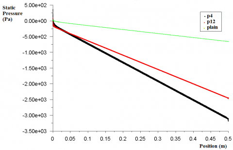
Figure 16 shows, as a comparison, the pressure drop for L/D = 4, L/D = 12 and for the pipe without insert, as a function of axial distance from the input section.
5.2 Thermal analysis
The thermal analysis was performed by controlling the temperature field for different sections of the pipe, detecting, in particular, the wall and bulk temperatures.
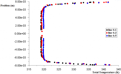
Figure 17 shows the temperature profiles as a function of axial distance, for the same sections shown in Figure 13.
The CFD analysis performed, varying the twist ratio, by imposing a wall heat flux of Φext=5,000 W/m2 and a mass flow rate of crude oil $\dot{m}$=0.041 kg/s with an inlet temperature Tin = 319 K, provide a value of the outlet temperature, Tout, of about 321 K. At the same result (Tout = 320.6 K) is reached theoretically by Eq. (2) that, for the energy conservation equation Eq. (1), is independent of both the presence of the turbulator and its twist ratio.
Figure 18 shows the temperature field in correspondence to the surface of the pipe.
Figure 16. Pressure drop for a pipe without insert and for twist ratio of 4 and 12
Figure 17. Trend of temperature (L/D=4)
Figure 18. Temperature field in correspondence to pipe surface
The wall temperature, owing to the condition of constant heat flux, increases with the twist ratio of the turbulator because of the lower heat removal from the fluid.
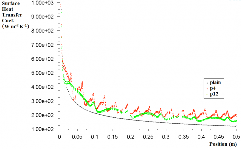
Figure 19 shows the local convective heat transfer coefficient for the pipe provided with turbulator with a twist ratio L/D = 4 and L/D = 12 and for the pipe without insert (plain).
Figure 19 shows the effective increase in the convective heat transfer coefficient h to decrease the twist ratio of the turbulator (increase of induced turbulence) compared to the case of the pipe without insert. Because of the swirl motion induced, the wall temperature of the pipe is not presenting a uniform trend. Since the removal of heat is greater in areas where the fluid is more susceptible to the effect of the insert, the flow will not be one-dimensional, but oscillating between a minimum and maximum value, with effect on the value of h. This phenomenon is shown in the periodic trend of the convective heat transfer coefficient, as shown in Figure 19. From the same figure it is possible to note, moreover, how the frequency of the oscillations decreases with increasing twist ratio, tending to infinity for the case corresponding to the pipe without insert.
Table 5 reports the average values of the wall temperature and of the convective heat transfer coefficient. The table shows, as already mentioned, that increasing the twist ratio causes the increase in the wall temperature and the decrease in the convective heat transfer coefficient h. It is interesting to note that the increase in this coefficient, compared to the case of a pipe without insert, is between 30 % (L/D = 16) and 81 % (L/D = 2).
Figure 19. Local convective heat transfer coefficient
Table 5. Average values of the convective heat transfer coefficient and the wall temperature to vary the twist ratio of the turbulator
|
L/D |
$\overline{T}_{w}$[K] |
$\overline{h}$[W/m2 K] |
|
2 |
335.98 |
294.46 |
|
4 |
339.83 |
240.04 |
|
6 |
341.09 |
226.35 |
|
8 |
341.56 |
221.63 |
|
10 |
342.03 |
217.13 |
|
12 |
342.23 |
215.26 |
|
14 |
342.30 |
214.56 |
|
16 |
342.47 |
213.03 |
|
Plain |
349.78 |
162.44 |
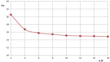
Figure 20 reports the trend of the Nusselt number to vary the twist ratio of the turbulator. It decreases when the twist ratio increases, assuming values greater than those relative to the pipe without insert (Nu = 4.36).
Taking into account that the thermal profile for the 500 mm pipe is not definitely developed, other CFD simulations were conducted by imposing the condition of translational periodicity between input and output sections, in order to determine the average values of the convective heat transfer coefficient. These data are reported in Table 6.
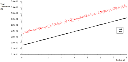
In the simulations carried out on the 500 mm pipe, because of its reduced axial dimension, it was possible to neglect the influence of temperature on the thermo-physical properties of the fluid. For a better understanding of the problem and of the behaviour of the fluid in the case of large temperature differences between input and output section, and to perform a comparison with a real case, the CFD analysis was applied to an 8-metre long pipe, provided with an insert with a twist ratio L/D = 8, with crude oil as working fluid and constant thermal flux on the wall equal to 1,257 W/m2. In the solver, the laws of variation of thermo-physical properties, according to those shown in Table 3, were set. The wall and bulk temperatures, shown in Figure 21, have the same trend as reported in the literature in reference [9]. The periodicity of the wall temperature (cloud of points in red) is observed also for this geometry. The results obtained from CFD analysis applied to the pipe without turbulator confirm the theory of Nusselt. In fact, a value of Nusselt close to that furnished by Eq. (4) is achieved for this situation.
A comparison with a real exchanger designed using the HTRI software could be made for this geometry. The software also provides the average value of the convective heat transfer coefficient. The comparison shows that the average value of h obtained with the CFD analysis, equal to 217.51 W/m2, is 7 % higher than that provided by HTRI software (203.89 W/m2). The pressure losses, however, are calculated with a standard deviation of less than 1 %. This variation could be attributed to the hypothesis of a constant heat flux on the wall used in CFD analysis that certainly does not occur in the real condition.
The simulations conducted with HTRI software have shown that the best trade-off design solution, which takes into account the efficiency of the heat exchange, the pressure losses, the overall dimensions, etc., is obtained with a twist ratio equal to 8.
Table 6. Average values of h at varying of the twist ratio
|
L/D |
6 |
8 |
10 |
12 |
14 |
16 |
Plain |
|
$\overline{h}$ |
229.68 |
200.13 |
181.06 |
166.76 |
154.94 |
146.00 |
39 |
Figure 20. Trend of Nusselt number as a function of twist ratio
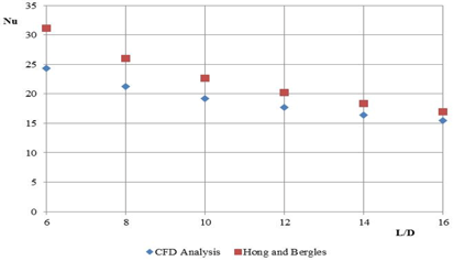
The values of the Nusselt number obtained from CFD analysis for the pipe with thermal profile settled in which the heavy oil is used, were compared with the values obtained by the correlation of Hong and Bergles [3], valid, as reported by Saha and Dutta [10], until Pr = 730.
$\mathrm{Nu}=0.383 \mathrm{Pr}^{0.35}\left(\frac{\mathrm{Re}}{L / 2 D}\right)^{0.622}$(4)
The results of the comparison are shown in Table 7 and in Figure 22.
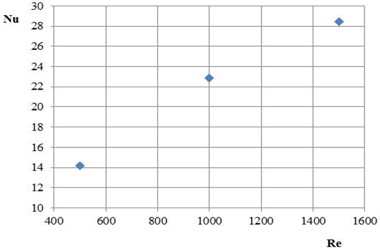
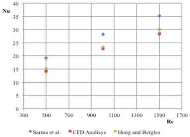
In order to evaluate the average convective heat transfer coefficient to vary the Reynolds number, the CFD analysis was performed for a 1500 mm long pipe with a twist ratio L/D=8, using water as working fluid. The complete development of thermal and hydrodynamic boundary layer occurs for this length. The Nusselt number was rated for Reynolds numbers of 500, 1,000 and 1,500 (Figure 23). These results were compared with those obtained from the application of Eq. (4) and Eq. (5) proposed by Sarma et al. [4], valid for water (Pr=7), as shown in Figure 24 and in Table 8. Moreover, the differences are shown between the values supplied by the correlations and those obtained with the CFD analysis in this assessment.
$\mathrm{Nu}=0.2036\left[1+\frac{\mathrm{D}}{\mathrm{L}}\right]^{4.12} \mathrm{Re}^{0.55} \mathrm{Pr}^{\frac{1}{3}}$(5)
Figure 21. Trend of the temperature of the bulk and of the wall
Table 7. Comparison between CFD analysis and correlation of Hong and Bergles for the pipe with settled thermal profile
|
L/D |
Nusselt number |
||
|
CFD analysis |
Hong and Bergles |
Error |
|
|
6 |
24.37 |
31.16 |
22 % |
|
8 |
21.23 |
26.06 |
19 % |
|
10 |
19.21 |
22.68 |
15 % |
|
12 |
17.69 |
20.25 |
13 % |
|
14 |
16.44 |
18.40 |
11 % |
|
16 |
15.49 |
16.93 |
9 % |
Figure 22. Comparison between CFD analysis and correlation of Hong and Bergles for the pipe with settled thermal profile
Figure 23. Nusselt number as a function of the Reynolds number
Figure 24. Comparison between the correlations of Sarma, Hong and Bergles and CFD analysis for a 1 500 mm long pipe
Table 8. Comparison between the correlations of Sarma, Hong and Bergles and CFD analysis for a 1,500 mm long pipe
|
Nusselt number |
Percentage difference |
||||
|
Re |
Sarma et al. |
Hong and Bergles |
CFD analysis |
Sarma et al. |
Hong and Bergles |
|
500 |
19.30 |
15.25 |
14.20 |
26 % |
7 % |
|
1,000 |
28.26 |
23.47 |
22.84 |
19 % |
3 % |
|
1,500 |
35.32 |
30.20 |
28.42 |
20 % |
6 % |
In this paper a pipe provided with inserts of twisted tape type was analyzed by CFD analysis and by varying the twist ratio. Using this system it is possible to increase the convective heat transfer coefficient due to the induced swirl motion which improves the mixing of the fluid and allows a greater heat removal.
The analysis carried out on a 500 mm long pipe provided with turbulator showed a significant increase in the convective heat transfer coefficient compared to the case of pipe without an insert. Using crude oil as the working fluid, the increase is between 30 % (L/D = 16) and 81 % (L/D = 2). The reduction of the twist ratio causes an increase in the heat exchange but also an increase in the pressure losses, relevant for certain cases. In the design phase it is necessary to choose a trade-off between the allowable pressure losses and the power to be exchanged. It was found that this condition is verified by the configuration of turbulator with twist ratio equal to 8.
The analysis for a real exchanger with 8 m long pipes, designed with the aid of the HTRI software, showed a difference of 7 % on the average value of h and a deviation of less than 1 % for the pressure losses compared to CFD analysis.
Finally, a comparison was made with some correlations in the literature using both crude oil and water as working fluids. The correlation of Hong and Bergles, compared to the results provided by the CFD analysis, present a good agreement when the working fluid is water and presents a mean deviation of 5.3 %. However, the same correlation present an average difference of 15 % when the working fluid is crude oil.
The correlation of Sarma et al., valid only for water, returns results which differ by 21.6 % from those supplied by CFD analysis.
|
cpinc |
specific heat of Incoloy-825, J. kg-1. K-1 |
||
|
cpco |
specific heat of crude oil, J. kg-1. K-1 |
||
|
D |
width of tape, mm |
||
|
h |
convective heat transfer coefficient, W.m-2.K-1 |
||
|
$\overline{h}$ |
average convective heat transfer coefficient, W.m-2.K-1 |
||
|
kinc |
thermal conductivity of Incoloy-825, W.m-1.K-1 |
||
|
kco |
thermal conductivity of crude oil, W.m-1.K-1 |
||
|
l |
pipe length, m |
||
|
L |
tape length, mm |
||
|
L/D |
twist ratio, dimensionless |
||
|
$\dot{\mathrm{m}}$ |
water flow rate, g.s-1 |
||
|
Nu |
Nusselt number, dimensionless |
||
|
Pr |
Prandtl number, dimensionless |
||
|
Qext |
external heat power, W |
||
|
Qin |
input heat power, W |
||
|
Qout |
output heat power, W |
||
|
Re |
Reynolds number, dimensionless |
||
|
RMSEP |
root mean squared percentage error, % |
||
|
s |
thickness of the pipe, mm |
||
|
Tin |
temperature in the inlet section, °C |
||
|
Tout |
temperature in the outlet section, °C |
||
|
$\overline{T}_{w}$ |
average temperature of the wall, °C |
||
|
Greek symbols |
|||
|
δ |
thickness of the tape, mm |
||
|
Δp |
pressure drop per unit length, Pa.m-1 |
||
|
μco |
dynamic viscosity of crude oil, N.s.m-2 |
||
|
ρinc |
density of Incoloy-825, kg.m-3 |
||
|
ρco |
density of crude oil, kg.m-3 |
||
|
$\varphi_{\mathrm{ext}}$ |
external diameter of the pipe, mm |
||
|
Φext |
external heat flux, W.m-2 |
||
|
Subscripts |
|||
|
co |
crude oil |
||
|
ext |
external |
||
|
in |
inlet |
||
|
inc |
Incoloy-825 |
||
|
out |
outlet |
||
|
w |
wall |
||
[1] P. K. Sarma, T. Subramanyam, P. S. Kishore, V. D. Rao and S. Kakac, “Laminar convective heat transfer with twisted tape inserts in a pipe,” International Journal of Thermal Science, vol. 42, pp. 821-828, 2003. DOI: 10.1016/S1290-0729(03)00055-3.
[2] A. Galloro, R. Schimio, N. Palmieri and S. Barbieri, “Comparazione tecnico-economica di uno scambiatore di calore a fascio tubiero in presenza di un fluido viscoso nel lato tubi mediante l’utilizzo di inserti meccanici interni ‘Twisted Tape’ con differenti passi di torsione,” in Proc. of VIII National Congress of AIGE, Reggio Emilia, Italy, 9 June 2014.
[3] S. W. Hong and A. E. Bergles, “Augmentation of laminar flow heat transfer in tubes by means of twisted tape inserts,” ASME J. Heat Transfer, vol. 98, pp. 251-256, 1976. DOI: 10.1115/1.3450527.
[4] P. K. Sarma, P. S. Kishore, V. D. Rao and T. Subrahmanyam, “A combined approach to predict friction coefficients and convective heat transfer characteristics in a tube with twisted tape inserts for a wide range of Re and Pr,” International Journal Of Thermal Science, vol. 44, pp. 393-398, 2005. DOI: 10.1016/j.ijthermalsci.2004.12.001.
[5] A. Galloro, R. Schimio and L. Danziani, “Ottimizzazione tecnico-economica di uno scambiatore di calore a fascio tubiero mediante l’utilizzo di inserti meccanici interni”, in Proc. of VII National Congress of AIGE, Rende (CS), Italy, 10-11 June 2013.
[6] A. Dewan, P. Mahanta, K. Sumithra Raju and P. Suresh Kumar, “Review of passive heat transfer augmentation techniques,” Journal of Power and Energy Proceedings of the Institution of Mechanical Engineers, vol. 218, Part A, pp. 509-527, 2004. DOI: 10.1243/0957650042456953.
[7] K. Sivakumar and K. Rajan, “Experimental analysis of heat transfer enhancement in a circular tube with different twist ratio of twisted tape inserts,” International Journal of Heat and Technology, vol. 33, no. 3, pp. 158-162, 2015. DOI: 10.18280/ijht.330324.
[8] R. M. Manglik and A. E. Bergles, “Heat transfer and pressure drop correlations for Twisted tape inserts in Isothermal tubes: Part I-Laminar flows,” ASME Journal of Heat Transfer, vol. 115, pp. 881-889, 1993. DOI: 10.1115/1.2911383.
[9] William M. Kays and H. C. Perkins, “Forced convection, internal flow in ducts”, in Warren M. Rohsenow and James P. Hartnett, Handbook of Heat Transfer, New York: McGraw Hill, 1973, pp. 7.19-7.27.
[10] S. K. Saha and A. Dutta, “Thermohydraulic study of laminar swirl flow through a circular tube with Twisted Tape,” ASME Journal of Heat Transfer, vol. 123, pp. 417-427, 2001. DOI: 10.1115/1.1370500.
[11] http://www.calgavin.com/heat-exchanger-solutions/hitran-systems/how-hitran-works/, Calgavin Limited Minerva Mill, Station Road, Alcester, Warwickshire B49 5et, UK.