OPEN ACCESS
A numerical simulation based on CDF/CSD methods is conducted to investigate the transonic static aeroelastic issues of large aircraft. The RANS equation and structural statics equations are utilized as governing equations to do coupling iterative calculation. In order to improve the accuracy and efficiency of CFD, multi-block structured grids are employed for parallel computation and the multi-grid method is used to accelerate convergence. Additionally, a dynamic mesh generation technique, based on a radial basis function (RBF) and the transfinite interpolation (TFI) method is adopted to enhance the efficiency and robustness of grid deformation. Moreover, a thin plate spline interpolation technique of three dimensions is utilized to improve the efficiency of data interpolation, coupled with the calculation of structural deformation based on the virtual work principle. The effectiveness of methods used in this paper is validated by a calculation example employing a static aeroelastic model of a wing-body configuration and independently developed software. Based on static aeroelastic analysis of this model in a typical region of transonic Mach number, several suggestions on static aeroelastic correction of large aircraft’s aerodynamic coefficients or derivatives can be given.
CFD/CSD, Static Aeroelasticity, Numerical Simulation, High-aspect-ratio Wing, Transonic Speed.
Static aero-elastic effect is an aerodynamic phenomenon that aerodynamic loads can be influenced by the structural deformation of flight vehicles induced by aerodynamic loads. In order to increase the lift-to-drag ratio, drag-divergence Mach number and the cruise speed in a transonic range, modern large aircraft generally utilize a high-aspect-ratio, supercritical and swept wing. Besides, the fuselage, wing and other main components are manufactured using new-style composite materials to reduce the weight of the aircraft. Although these measures can improve the aerodynamic performance and structure efficiency of large aircraft, static aeroelastic deformation of wing and other components will become more serious. Therefore, a huge number of studies have been conducted in order to predict the influence of aeroelasticity on aerodynamic performances and the structure safety of the aircraft more precisely [1-5].
In previous studies, due to restrictions on the calculation method and calculation conditions, the static aeroelastic characteristics of an aircraft were mainly estimated based on the linearized aerodynamic theory. For example, the solution of aerodynamic forces is based on the theory of linear small disturbance in NASTRAN which is software widely used in engineering applications, but only available for subsonic and low supersonic flow, where the conditions are not dominated by viscous and aeroelastic calculation of simple geometries [6-8]. However, as for the transonic flow of complex geometries such as a supercritical wing with divergent trailing
edge (DTE) aerofoil, and nacelle and control surfaces, a great difference can be found between the results of the aerodynamic forces solved by traditional methods and real results due to the nonlinearity of aerodynamic loads, flow separation induced by shock and boundary layer interference, and complex nonlinear aerodynamic phenomena including the interaction of aerodynamic loads of different aircraft components.
Since the 1980s, it has become increasingly possible to obtain accurate numerical solutions of critical transonic aeroelastic issues of flight vehicles because of the development of computational fluid dynamics (CFD) and computational structural mechanics (CSD), in particular CFD numerical simulation technology based on the Euler and Reynolds averaged Navier-Stokes (RANS) equations [9-13]. Nevertheless, as for modern advanced large aircraft, the number of grids for CFD calculation is extremely large, owing to the complex configuration and high accuracy requirements for the calculation of the transonic aerodynamic forces. Besides, static aeroelastic calculation is a process of repeated coupling iterative computation between flow field and structure, so it is difficult to apply in engineering for a calculation method based on a RANS equation because of its relatively low efficiency [14].
To solve transonic static aeroelastic problems of modern large aircraft with higher accuracy and efficiency, this paper provides a method that uses the RANS equation coupled with a structural statics equation based on previous investigations in the static aeroelastic calculation field. In order to improve the calculation accuracy and efficiency of the RANS equation, multi-block structured grids were carried out for parallel computation and multi-grid technology was adopted to accelerate convergence. In addition, the structural deformation was solved by static equilibrium equations based on flexibility matrix. Compared with solving structural modal motion equations, it could not only reduce solution variables but also save calculation time without reducing its accuracy. Moreover, in order to improve the efficiency and robustness of grid deformation, a dynamic grid generation technique based on radial basis function (RBF) and transfinite interpolation (TFI) was utilized. In addition, the dimension of the interpolation matrix was reduced through a greedy algorithm, which can reduce the total number of CFD iterations without changing the topology and the number of cells in the process of grid deformation by means of using the CFD calculation results of the previous step as the initial flow field values of the next step. Furthermore, the thin plate spline (TPS) interpolation technique was employed using the principle of virtual work to conduct data interpolation and structure deformation at the same time, which further improved the efficiency of the calculation.
To verify the validity of above methods, static aeroelastic numerical simulation was conducted based on a large wing-body aircraft model, and numerical as well as wind tunnel test results of several typical conditions were compared. Additionally, this paper investigated transonic static aeroelastic problems of this wing-body model in particular, and several suggestions on static aeroelastic correction of aerodynamic coefficients or derivatives were given.
2.1 CFD method
3D time-correlated conservative compressible RANS equations are used as governing equations. In general curvilinear coordinate system (ξ, η, ζ), the dimensionless form is
$\frac{\partial \boldsymbol{Q}}{\partial t}+\frac{\partial\left(\boldsymbol{F}-\boldsymbol{F}_{v}\right)}{\partial \xi}+\frac{\partial\left(\boldsymbol{G}-\boldsymbol{G}_{v}\right)}{\partial \eta}+\frac{\partial\left(\boldsymbol{H}-\boldsymbol{H}_{v}\right)}{\partial \zeta}=0$ (1)
Where, t is the time, Q is the conservation variable and F, G and H are inviscid flux terms. Fv, Gv and Hv represent the viscous flux terms.
The calculation is based on the finite volume method and the convection term utilizes Roe’s upwind flux-difference-splitting method for discretization. Also, a Venkat limiter is introduced to suppress the non-physical oscillation near shock waves and Van Leer’s Monotone Upstream-Centered Schemes for Conservation Laws (MUSCL) are used for the interpolation of the conservation variables of the flow field. In addition, viscous terms are discretized using a 2-order central difference scheme and an implicit LU-SGS (Lower-Upper Symmetry Gauss-Seide) method is utilized for time difference. Moreover, the one-equation SA (Spalart-Allmaras) model is chosen as the turbulence model, the object wall adopts an adiabatic and non-slip boundary condition, the far field is a pressure far field using non-reflecting boundary condition and the multi-grid technique is applied to accelerate the convergence of the calculation.
2.2 CSD method
For linear elastic problems, the matrix of flexibility influence coefficients can be used to solve the structural statics equation, which avoids solving complicated structural modal motion equations. However, structural elastic deformation can actually be obtained by several matrix operations, whose calculation time is shorter and processing is simpler and more suitable for studies of static aeroelastic problems. Generally, the elastic deformation of the wing is only considered in the process of static aeroelastic calculation of large aircraft and some other components such as fuselage, engine or hangings are assumed as rigid parts. The wing’s matrix of flexibility influence coefficients can be obtained by a structural finite element modeling calculation using MSC, NASTRAN or some other commercial software. Besides, it also can be directly achieved by test measurements. If aerodynamic loads, engine thrust and the mass force of three directions acting on the wing structure are known, the elastic deformation displacement of structural points can be obtained based on the structural equation whose form is
$\mathrm{u}_{\mathrm{s}}=\boldsymbol{C} \boldsymbol{F}_{s}$ (2)
Here, us is the deformation displacement vector of structure points, C is flexibility matrix of the structure points, and FS is mass force of aerodynamic loads, engine thrust and mass force acting on the structure points.
2.3 Interpolation method between flow field and structure
CFD calculation of conventional static aeroelastic issues is based on the Euler coordinate system and CSD is described based on the Lagrange coordinate system. Therefore, the division of the CFD grid and construction of the structure model are independent, so data exchange needs to be introduced between the structure and the flow field. One method is to transform the displacement of structure points to that of grid points; a second method is to transform the aerodynamic loads of CFD grid points to an equivalent force acting on structure points. As for static aeroelastic calculation, its deformation of three-dimensional space is small, so it is more suitable to use a three-dimensional TPS method in consideration of the memory occupancy rate, calculating its efficiency and precision of interpolation [15].
In the TPS method, the structure displacement interpolation matrix H can be obtained through the coordinates of the CFD grids and structure points of the flexibility matrix. Define that us and ua are the deformation shift vector of the structure points and deformation shift vector of CFD grid points respectively, then
$\boldsymbol{u}_{\mathrm{a}}=\boldsymbol{H} \boldsymbol{u}_{\mathrm{s}}$ (3)
According to the virtual work principle, the interpolation matrix between the aerodynamic loads and the displacement interpolation matrix between structural grids and CFD grid points are transposed, which means
$\boldsymbol{F}_{\mathrm{s}}=\boldsymbol{H}^{\mathrm{T}} \boldsymbol{F}_{\mathrm{a}}$ (4)
Therefore, the deformation shift vector ua can be achieved through the equations (2) ~ (4) if aerodynamic loads of CFD surface grids Fa are known
$\boldsymbol{u}_{\mathrm{a}}=\boldsymbol{H} \boldsymbol{C} \boldsymbol{F}_{\mathrm{s}}=\boldsymbol{H} \boldsymbol{C} \boldsymbol{H}^{\mathrm{T}} \boldsymbol{F}_{\mathrm{a}}$ (5)
2.4 Dynamic mesh generation method
It is apparent that previous CFD grids are no longer applicable because of the deformation of the object surface, so new grids must be generated. There are two methods to generate new grids. One is through regenerating the grid directly, whose computational efficiency is quite low and is likely to change the mesh topology and the number of grid cells. The other method is through adding an amount of correction to the previous mesh. Due to the static aeroelastic calculation being based on an assumption that the structural deformation is small and the deformation of the structure in the local area is usually not severe, the second method is feasible and applied extensively, and its computational efficiency is relatively higher. This paper integrates the RBF and TFI methods to generate dynamic structure grids.
The RBF method is a volume interpolation based on spline function and also can be regarded as the expansion in three dimensions of the surface spline function interpolation method [16]. Its interpolation formula is
$f(\boldsymbol{r})=\sum_{i=1}^{n} a_{i} \varphi\left(\left\|\boldsymbol{r}-\boldsymbol{r}_{i}\right\|\right)+\psi(\boldsymbol{r})$ (6)
Here, $\boldsymbol{r}_{i}=\left(x_{i}, y_{i}, z_{i}\right)$ are points whose displacements are known and their number is n. In addition, φ is the primary function of space distance $\left\|r-r_{i}\right\|$ . In this paper, $\varphi\left(\left\|\boldsymbol{r}-\boldsymbol{r}_{i}\right\|\right)=\left\|\boldsymbol{r}-\boldsymbol{r}_{i}\right\|^{3}$ , $\psi=b_{0}+b_{1} x+b_{2} y+b_{3} z$ . The coefficients of the interpolation equation can be obtained through displacement di of riand equilibrium condition
$f\left(r_{i}\right)=d_{i}$
$\sum_{i=1}^{n} a_{i}=\sum_{i=1}^{n} a_{i} x_{i}=\sum_{i=1}^{n} a_{i} y_{i}=\sum_{i=1}^{n} a_{i} z_{i}$ (7)
Their matrix forms are
$\left[\begin{array}{cc}\boldsymbol{\Phi} & \boldsymbol{P} \\ \boldsymbol{P}^{\mathrm{T}} & 0\end{array}\right]\left[\begin{array}{l}\boldsymbol{a} \\ \boldsymbol{b}\end{array}\right]=\left[\begin{array}{l}\boldsymbol{d} \\ 0\end{array}\right]$
$\boldsymbol{\Phi}=\left[\begin{array}{cccc}\varphi_{11} & \varphi_{12} & \mathrm{L} & \varphi_{1 n} \\ \varphi_{21} & \varphi_{22} & \mathrm{L} & \varphi_{2 n} \\ \mathrm{M} & \mathrm{M} & \mathrm{O} & \mathrm{M} \\ \varphi_{n 1} & \varphi_{n 2} & \mathrm{L} & \varphi_{n n}\end{array}\right]$ (8)
Where,
$P=\left[\begin{array}{llll}1 & x_{1} & y_{1} & z_{1} \\ 1 & x_{2} & y_{2} & z_{2} \\ \mathrm{M} & \mathrm{M} & \mathrm{M} & \mathrm{M} \\ 1 & x_{n} & y_{n} & z_{n}\end{array}\right]$ ,
$\boldsymbol{a}=\left[\begin{array}{c}a_{1} \\ a_{2} \\ \mathrm{M} \\ a_{n}\end{array}\right]$ ,$\boldsymbol{b}=\left[\begin{array}{l}b_{0} \\ b_{1} \\ b_{2} \\ b_{3}\end{array}\right]$ and $\boldsymbol{d}=\left[\begin{array}{c}d_{1} \\ d_{2} \\ \mathrm{M} \\ d_{n}\end{array}\right]$,
$\varphi_{i j}=\varphi\left(\left\|\boldsymbol{r}_{i}-\boldsymbol{r}_{j}\right\|\right)$ .
After obtaining the interpolation function coefficients, displacement dinter of any interpolation point rintercan be achieved: $\boldsymbol{d}_{\mathrm{int} e r}=f\left(\boldsymbol{r}_{\mathrm{int} e r}\right)$ .
Theoretically, the displacement of the whole space grid can be got directly by interpolation based on the primary function method, if the displacement of the surface grids is known and the displacement of the far field grid points is set to zero. However, the dimensions of matrixΦ in equation (8) will be too many and the calculation efficiency of grid deformation is quite low when the geometric configuration is complex and the number of surface grids is large. In order to improve the computational efficiency, this paper utilizes the greedy algorithm and only selects that part of the object surfaces as well as far-filed grids as points of the radial basis function whose coordinates are known in the process of interpolation using RBF, which can improve computational efficiency.
Based on the above methods, the displacement of the internal grid points of all grid blocks’ lines can be achieved through interpolation using the RBF method for dynamic grids, the displacement of internal surface grids of all grid blocks can be obtained by the TFI method [17] based on block surfaces’ lines and internal grid points in all blocks can be obtained by the TFI method based on the blocks’surfaces.
3.1 Calculation model and CFD grids
This paper carried out the static aeroelastic calculation of a wind tunnel test model that is a large wing-body aircraft; the results were compared with those of the wind tunnel test. The wing of this model used a supercritical wing with divergent trailing edge aerofoil and ignored the nacelle/pylon, flap track fairing and some other parts. Figure 1 shows the geometry and surface grids of the model. During the calculation, we only considered the influences of aerodynamic loads and deformation of the wing, and the fuselage only performed a function of rectification. The matrix of flexibility influence coefficients for the deformation calculation of the wing structure can be obtained through a ground test.
Figure1. Calculation model and its initial CFD grids
CFD initial grids are multi-block structured grids, which contain a layer of boundary layer grids enwrapping the fuselage and wing. The grid cell size is approximately 500 million and thickness of the first layer is 0.002mm and makes y+≈1 for all walls. In order to accelerate the convergence using multi-grid technique, the number of lines of all block surfaces should be set according to the 4n+1 law (n is the number of multi-grid level).
3.2 Calculation verification
Calculation conditions for validation are Ma=0.78, q=35kPa, Re =7.3×10⁶ and α = -4°~8°.
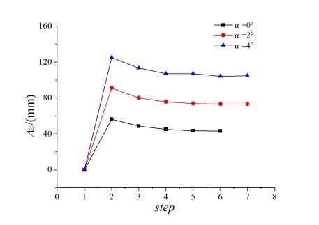
Static aeroelastic calculation is a process of repeated CFD/CSD coupling iterative calculation. For engineering applications, the efficiency of iterative calculation must be high and fast convergence speed is needed. As shown in figure 2, it only needs 6~7 deformation iterations for one calculation condition’s basal convergence based on methods provided in this paper. Besides, it does not change the topology and the number of cells in the calculation process, so the CFD calculation results of the previous step can be used as the initial flow field values of the next step. Generally, the computation amount of the CFD / CSD method in this paper is 1.5~2.0 times of that of the corresponding rigid model.
Figure 2. Iteration convergence curves of static aeroelastic deformation calculation
Comparison of the wing lift coefficient CL and bending deformation Δz (normal deformation of wing leading edge) between calculation and the corresponding wind tunnel test is shown in figure 3. What is worth mentioning is that CL in figure 3 had been conducted with some correlation corrections, including correction of the boundary layer transition simulation inconsistent, shape difference between the calculation model and the test model as well as wind tunnel wall interference. However, it is difficult to correct the influence of faulty turbulence simulation, inaccurate
separation simulation in the CFD calculation and nonlinearity of actual wing deformation at present. As a whole, the results of the calculation in this paper are completely consistent with those of the wind tunnel test. The difference of CL mainly occurs when flow is separated, primarily resulting from inaccurate CFD simulation. The difference of Δz mainly exists in the region of small deformation, which was probably induced by a larger measurement error in the small deformation situation.
(a) CL~α
(b) Δz~y/b
Figure 3. Comparison between results of numerical calculation and wind tunnel
In order to improve the aerodynamic efficiency of large aircraft, their cruise Ma is usually in the transonic range. So the viscous effect cannot be ignored due to shock and boundary layer interaction, even if the angle of attack is very small, and an N-S equation should be used. For not losing generality, the static aeroelastic effects of a wing-body model when Ma=0.78, were calculated as an example based on the methods provided in this paper.
4.1 Geometrical deformation characteristics
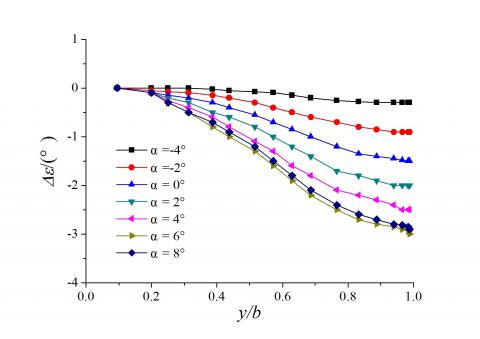
Figure 4 illustrates changes of Δz and Δε (torsion angle induced by static aeroelasticity) along span-wise direction when Ma=0.78, q=35kPa and α=-4°~8°. It can be seen from
figure 4 that the static aeroelasticity results in upward bending deflection deformation of the wing and negative elastic torsion angle in the downwind wing sections when the angle of attack is positive. In addition, it can be found that deformation of the inner wing is smaller, and deformation becomes larger away from the location where the wing is folded and peaks at the wing tip, which is consistent with the distribution characteristics of wing stiffness. As for swept wings, these kinds of deformation characteristics will reduce the local angle of attack of wing along the span-wise direction, affect the load distribution, and change their aerodynamic characteristics, which are so-called static aeroelastic effects. Taking the calculation result in this paper when Ma=0.78, q=35kPa, α=2° as an example, bending deformation of the wing tip is nearly 2% of the wing span and the elastic torsion angle and the change of α of wing tip sections can be about -2° and -4° respectively.
(a) Wing bending deformation
(b) Wing elastic torsion deformation
Figure4. Wing geometrical deformation characteristics
4.2 Surface pressure distribution characteristics
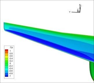
Figures 5 and 6 demonstrate the surface pressure distribution contours of rigid and elastic models as well as pressure coefficients of different span-wise sections separately when Ma=0.78, q=35kPa and α=2°. As can be seen from figure 6, static aeroelasticity has a small impact on the surface pressure of the wing root, and decreases the negative pressure range of the upper outboard wing obviously, as well as affecting the pressure distribution characteristics of the wing tip to a large extent; this is consistent with wing geometric deformation characteristics. Figure 6 shows that the differences of pressure distribution among different wing sections are not very large but the bias becomes increasingly larger for the wing sections closer to the wing tip. This is mainly because the aerodynamic loads of a swept wing result in upward bending deflection deformation of the wing, induce decrease of the downwind local angle of attack due to the negative elastic torsion angle, and reduce the suck peak of wing leading edge when the angle of attack of the wing is small and the upper wing does not appear to have a large area of flow separation. Taking the calculation result in this paper when Ma=0.78, q=35kPa, α=2° as an example, CL of an elastic wing is reduced by more than 15% compared with that of a rigid wing. Therefore, the impact of static aeroelasticity
on aerodynamic loads cannot be ignored for a high-aspect-ratio swept wing in a transonic speed range and must be underlined in the aircraft design stage.
(a) Rigid model
(b) Elastic model
Figure 5. Effects of static aeroelasticity on wing surface pressure
(a) y/b=20%
(b) y/b=60%
(c) y/b=95%
Figure 6. Comparison of pressure coefficients at different wing sections
4.3 Effect on aerodynamic characteristics and its correction
The dynamic pressure has a significant impact on the static aeroelastic effect of aircrafts. Therefore, the discipline as to how dynamic pressure affects the static aeroelastic correction factor of aerodynamic coefficients or derivatives needs to be studied.
Define
K=C_F/C_R (9)
Where, C_F and C_R represent aerodynamic coefficients or derivatives of an elastic wing and a rigid wing respectively. K is the correction factor of static aeroelasticity.
Define
K1=CLα-F/CLα-R
K2= $C_{m C_{L_{-}} F}$ / $C_{m C_{L_{-}} R}$
K3=Kα=2-F/ Kα=2-R (10)
Here, CLα, $C_{m C_{L}}$ and Kα=2 represent the slope of lift coefficient , longitudinal static stability margin and the lift-to-drag ratio of α=2o.
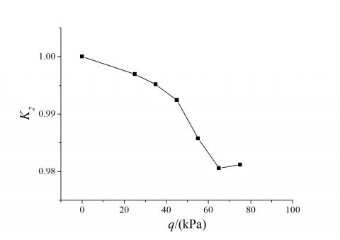
Figure 7 shows typical static aeroelastic correction factors of an elastic wing under different dynamic pressures when Ma=0.78. It can be seen that dynamic pressure has an impact on lift and drag characteristics as well as the static longitudinal stability of the elastic wing to different extents. Specifically, the slope of the lift coefficient K1 has basically a linear downward trend, whose value is approximately 0.94 when q=35kPa at cruise height. However, this kind of linear discipline will change after the dynamic pressure reaches one particular large value. As can be seen from figure 7(a), the curve of K1~q begins to upturn at q=65kPa, which probably results from geometrical nonlinearity of the wing elastic deformation when the dynamic pressure is relatively high. As for K2, the longitudinal static stability margin, it generally has a nonlinear downward trend with an increase of dynamic pressure. However, it is noticed from figure 7(b) that the characteristics of K2~q began to reverse when q>65kPa. Turning to K3, the lift-to-drag ratio of α=2o, static aeroelasticity will increase the lift-to-drag ratio as a whole, although it does decrease the lift due to the fact that it also reduces the drag induced by the lift. Figure 7 (c) demonstrates that linear characteristics can be found in K3 when dynamic pressure is low, but the nonlinearity is quite obvious after q>45kPa.
(a) K1~q
(b) K2~q
(c) K3~q
Figure7. Effects of static aeroelasticity on wing aerodynamic characteristics
In view of the above analysis, the probable nonlinearity of the static aeroelastic correction factor in high dynamic pressure should be considered and dynamic pressure range cannot be too small in calculation or experiment, in order to correct the static aeroelasticity of the high aspect ratio wing in transonic speed. Moreover, even if the dynamic pressure is low, its interval should not be too sparse in calculation, since some static aeroelastic correction factors of aerodynamic coefficients or derivatives may experience a nonlinear variation versus dynamic pressure. Therefore, considering both the reliability and economy of static aeroelasticity correction in a moderate or small angle of attack for large aircraft, a relatively reasonable way is by using the highly precise CFD/CSD method; however, the calculation method should be verified and corrected by a static aeroelastic wind tunnel test.
A CFD/CSD method for static aeroelasticitic calculation is developed in this paper, based on the RANS equation and structural static equation. In order to improve the accuracy and efficiency as much as possible, multi-block structured grids are employed for parallel computation, the multi-grid method is used to accelerate convergence, a dynamic mesh generation technique based on radial basis function (RBF) and transfinite interpolation (TFI) method is adopted, and the TPS interpolation technique is employed to conduct aerodynamic/structural data interpolation. Meanwhile, numerical simulation investigation is conducted based on this method, taking one static aeroelastic model of a wing-body configuration as a calculation example. The calculation results are consistent with the experimental data and proved to be efficient based on its iterative calculation process. Moreover, several suggestions on the static aeroelastic correction of a large aircraft’s aerodynamic coefficients or derivatives are given, based on the calculation results and static aeroelastic analysis of this model in a typical region of transonic Mach number.
1. HADDADPOUR H., KOUCHAKZADEH M.A., et al., “Aeroelastic instability of aircraft composite wings in an incompressible flow” [J], Composite Structures, 2008, 83(1): 93-99. DOI: 10.1016/j.compstruct.2007.04.012.
2. LIVNE E., WEISSHAAR T.A., “Aeroelasticity of nonconventional configurations: past and future” [J], Journal of Aircraft, 2003, 40(6):1047-1065. DOI: 10.2514/2.7217.
3. AHREM R., BECKERT A., WENDLAND H., “Recovering rotations in aeroelasticity” [J], Journal of Fluids and Structures, 2007, 23(6):874-884. DOI: 10.1016/j.jfluidstructs.2007.02.003.
4. SVACEK P., “Application of finite element method in aeroelasticity” [J], Journal of Computational and Applied Mathematics, 2008, 215(2):586-594. DOI: 10.1016/j.cam.2006.04.069.
5. ATTORNI A., CAVAGNA L., et al., “Aircraft T-tail flutter predictions using computational fluid dynamics” [J], Journal of Fluids and Structures, 2011, 27(2): 161-174. DOI: 10.1016/j.jfluidstructs.2010.11.003.
6. RODDEN W.P., JOHNSON E.H., MSC/Nastran Aeroelastic Analysis User’s Guide V68 [M], Los Angeles: MSC Software Corporation, 1994: 44-65.
7. NEILL D.J., HERENDEEN D.L., et al., ASTROS Enhancements, Vol.3: ASTROS Theoretical Manual [R], New York: AD-A308134, 1995.
8. ZONA, ZONAIR User Manual [M], Scottsdale, AZ85251-3540, 2005.
9. RAMJI K., WEI S., et al., “Time dependent RANS computation for an aeroelastic wing” [J], AIAA Paper, 2004-0886, 2004. DOI: 10.2514/6.2004-886.
10. ROBINSON B.A., BATINA J.T., et al., “Aeroelastic analysis of wings using the Euler equation with a deforming mesh” [J], Journal of Aircraft, 1991, 28(11):781-788. DOI: 10.2514/3.46096.
11. GURUSWAMY G.P., “Unsteady aerodynamic and aeroelastic calculations for wings using Euler equations” [J], AIAA Journal, 1990, 28(3):461-469. DOI: 10.2514/3.45715.
12. KENNETH E.T., GARY L.G., “Integration nonlinear aerodynamic and structural analysis for a complete fighter configuration” [J], Journal of Aircraft, 1988, 25(12): 1150-1156. DOI: 10.2514/3.45715.
13. SMITH M.J., PATIL M.J., HODGES D.H., “CFD-based analysis of nonlinear aeroelastic behavior of high-aspect ratio wings” [C], Seattle: AIAA, 2001-1528, 2001. DOI: 10.2514/6.2001-1582.
14. MA Y.F., HE E.M., et al., “Static aeroelastic analysis for high-aspect-ratio wing” [J], Aeronautical Computing Technique, 2005, 44(3): 53-57. (in Chinese) DOI: 10.3969/j.issn.1671-654X.2014.03.013.
15. LIU Y., BAI J.Q., et al., “An approach to CFD/CSD non-linear coupling based on RBF interpolation technology” [J], Chinese Journal of Computational Mechanics, 2014, 31(1): 120-127. (in Chinese) DOI: 10.7511/jslx201401021.
16. HOLGER W., “Computational aspects of radial basis function approximation” [J], Studies in Computational Mathematics, Vol. 12, 2006, pp. 231-256. DOI: 10.1016/S1570-579X(06)80010-8.
17. SONI B.K., “Two- and three-dimensional grid generation for internal flow applications of computational fluid dynamics” [C], 7th Computational Physics Conference, Cincinnati, OH, AIAA Paper 185-1526, 1985. DOI: 10.2514/6.1985-1526.