OPEN ACCESS
Two phase CFD calculations, using Eulerian-Lagrangian model with commercial Fluent 6.3 were employed to predict the gas and particle flow in pipe of complex geometry designed for pneumatic conveying of olive cake particles toward a pulverized burner. The numerical calculations were validated against experimental data from the literature. The effects of gas velocity and particles size distribution on the mixture flow behavior were studied. The present results help to understand the phenomena occurring in gas-solid flow and optimizing the conveying system.
pneumatic conveying system, two-phase flow, pipe bend, Eulerian-Lagrangian model, gas-particles flow.
The pneumatic transport of dilute suspensions of particles in gas flows through bends or elbows has many shortcomings and because of the change in flow direction [1]. One such problem is that the rope formation. Indeed, the mixture of gas–solid system makes a turn within an elbow; particles form a rope-like structure because of inertial effects [2]. Other problems such as bends erosion and particles fragmentation; these problems may cause breakdown of the plant or limit the use of the pneumatic conveying system [3].
Many investigators have carried out both experimental and numerical modelling of the transport phenomenon of the conveying process in gas–solid system within pipe bends, elbows, tees and related geometries. The flow profiles of the solids in the pipes of different sizes and for different pipe bends have been characterized in order to help on the optimization of the pneumatic conveying process and to assess the different methods of monitoring the conveying systems [4].
The formation and dispersion of ropes and gas-particles flow behavior through and after pipe bend have been studied numerically and experimentally by Yilmaz and Levy [2]. The results show a denser particle rope as the pipe bend radius to pipe diameter ratio is increased and secondary flows disperse the rope by carrying particles around the pipe circumference while turbulence disperses the rope by localized mixing of particles.
Gore and Crowe [5] have investigated the effect of the particles size on the flow behavior in a pipe. They have concluded that if the ratio of particles size by flow length scale (dp/Le) is less than 0.1 then the turbulence has reduced and else that has amplified. In other hand, the kinetic energy of the flow with gross particles is over then that of flow with small particles.
Based in many previous studies [2] [6-10], flow behavior of the conveying process in gas–solid system within pipe bends is much related to characteristic parameters of particles such as size, density and mass loading ratio and geometries configurations.
The objective of this article is to investigate the flow characteristics of two-phase flow conveying system and use it for the design and optimization of pulverized solid-olive-waste burners.
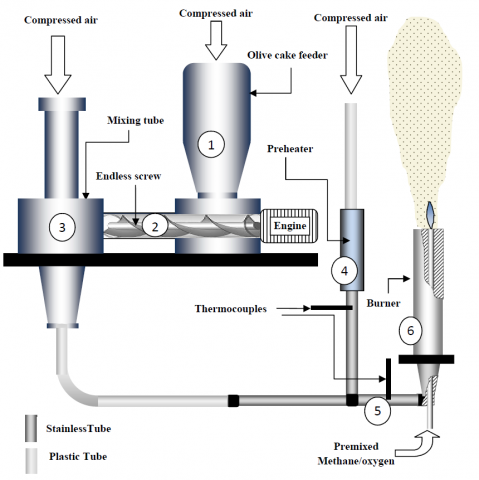
A new pilot plant is designed and installed in order to produce pulverized jet flame of olive cake. The experiment principle consists to produce a jet of air diluted with olive cake particles having sizes inferiors or equals to 200 μm discharged in free air. The pulverized jet flame is ignited by a pilot flame. Figure 1 shows the schematic diagram of the pilot plant used for pulverized olive cake combustion.
The circulation of olive cake particles through the pneumatic conveying system until burner is described below:
The olive cake particles are initially stored in the reservoir (1). Then, they are drove by an endless screw (2) towards mixing pipe (3). Compressed air is injected into the particles feeder (1) with an aim to improve the particles drive. Another flow rate of compressed air is injected in tube (3) in order to entrain the particles towards the burner (6). If the preheating is selected, a hot air coming from the preheater (4) should be mixed with the cold mixture of air /olive cake. In the both case, the mixture of air /olive cake goes in the burner (5). The main injector pipe (5) has an inner diameter of 30 mm and a height of 300 mm. The mixture of air/olive cake passes through tubes with different geometry before being introduced in the straight main injector pipe. Each gas line is consisted by the following essential elements assembled in series: a valve, a pressure regulator, a manometer and a colsonic.
Figure 1. Schematic diagram of the pilot plant used for pulverized olive cake combustion
Properties of olive cake are illustrated in table 1.
Table 1. Properties of olive cake (Sample comes from the Tunisian Sahel region 2011)
|
Parameter |
Value |
|
|
Ultimate analysis |
Carbon |
47.15 wt% |
|
Hydrogen |
6.03 wt% |
|
|
Oxygen* |
41.3 wt% |
|
|
Nitrogen |
1.34 wt% |
|
|
Sulfur |
< wt1% |
|
|
Moisture** |
1.85 wt% |
|
|
Oil content** |
2.25 wt% |
|
|
Ash |
2.36 wt% |
|
|
LHV |
17510 kJ/kg |
|
|
Density |
565 kg/m3 |
|
* Value determined by difference
**Analysis carried out just after drying phase
The aim of this work is to predict the mixture flow (olive cake and air) in pipe of conveying system.
Eulerian/Lagrangian approach is used to describe the flow and particle motion. Then, Eulerian frame was employed to formulate the continuous phase equations, while simulating the discrete phase in the Lagrangian frame.
3.1 Governing equation for gaseous phase
The gas-phase time-averaged continuity equation and conservation equations of momentum can be written as:
$\frac{\partial \rho \bar{u}_{i}}{\partial x_{j}}=0$ (1)
$\frac{\partial \rho \bar{u}_{i} \bar{u}_{j}}{\partial x_{j}}=-\frac{\partial \bar{p}}{\partial x_{i}}+\frac{\partial}{\partial x_{j}} \mu\left[\frac{\partial \bar{u}_{i}}{\partial x_{j}}+\frac{\partial \bar{u}_{j}}{\partial x_{i}}\right]-\frac{\partial}{\partial x_{j}}(\rho \overline{u_{i}^{\prime} u_{j}^{\prime}})+\rho g_{i}+\bar{F}_{i}$ (2)
Additional terms (so-called Reynolds stresses) appear that represent the turbulence effects. In order to close averaged equations, these Reynolds stresses must be modeled.
The commercial CFD software FLUENT 6.3 is used to solve the Reynolds Averaged Navier- Stokes (RANS) equations for continuous gas phase. In the commercially FLUENT software the conservation equations of mass and momentum are discretized using the finite volume method. Second-order upwind algorithms were used to solve the continuity and momentum equations. Pressure was solved by PRESTO! Algorithm (PREssure STaggering Option procedure) and SIMPLE scheme were adopted for coupling between the pressure and velocity.
The resulting equations system is closed using the standard κ-e turbulence model. From a practical point of view, the use of the steady-state Reynolds-averaged Navier Stokes (RANS) equations closed by the standard κ-$\varepsilon$ turbulence model equations is cost-effective because it reduces the required computational effort and resources, and is widely adopted for the prediction of the flow behavior [12-14]. The standard κ-e turbulence model adopts a turbulent eddy viscosity by using the Boussinesq hypothesis and it leads to two additional transport equations: The turbulence kinetic energy κ and the turbulence dissipation rate $\epsilon$.
For a steady state, the transport equations of the turbulence kinetic energy κ and the turbulence dissipation rate e are expressed by:
$\frac{\partial \rho \kappa \bar{u}_{i}}{\partial x_{i}}=\frac{\partial}{\partial x_{j}}\left[\left(\mu+\frac{\mu_{t}}{\sigma_{\kappa}}\right) \frac{\partial \kappa}{\partial x_{j}}\right]+G_{\kappa}-\rho \epsilon$ (3)
$\frac{\partial \rho \epsilon \bar{u}_{i}}{\partial x_{i}}=\frac{\partial}{\partial x_{j}}\left[\left(\mu+\frac{\mu_{t}}{\sigma_{\epsilon}}\right) \frac{\partial \epsilon}{\partial x_{j}}\right]+C_{1 \epsilon} \frac{\epsilon}{\kappa} G_{\kappa}-C_{2 \epsilon} \rho \frac{\epsilon^{2}}{\kappa}$ (4)
Where $G_{\kappa}$ is the generation of turbulence kinetic energy due to the mean velocity gradients:
$G_{\kappa}=\mu_{t}(\sqrt{2 S_{i j} S_{i j}})^{2} ; S_{i j}=\frac{1}{2}\left(\frac{\partial \bar{u}_{i}}{\partial x_{j}}+\frac{\partial \bar{u}_{j}}{\partial x_{i}}\right)$ (5)
The turbulent viscosity is computed as a function of κ and ϵ:
$\mu_{t}=\rho C_{\mu} \frac{\kappa^{2}}{\epsilon}$ (6)
The turbulence model constants are listed in Table 2:
Table 2. Turbulence model constants
|
Constant |
$C_{\mu}$ |
$C_{1 \epsilon}$ |
$C_{2 \epsilon}$ |
$\sigma_{\kappa}$ |
$\sigma_{\epsilon}$ |
|
Value |
0.09 |
1.44 |
1.92 |
1.0 |
1.3 |
Particles are considered as solid spheres which are injected into the computational domain via surface injection model. The inter-phase mass and momentum exchanges are incorporate during simulations by using source terms in the Eulerian gas-phase equations. The Two-way coupling model is adopted.
3.2 Particle motion
In the Lagrangian computation of the dispersed phase model, the position and the velocity of a particle are $x_{p}$ and $v_{p}$, respectively.
In this study, all discrete particles are assumed spherical and intra-particle heat and mass transfer are not included in the discrete phase particle computation. The trajectory of a discrete phase particle is predicted by integrating the force balance on the particle. For small heavy particles in the dilute regime, drag and inertia effects are dominating forces [15]. Consequently, the motion equation of a particle can be written as:
$\frac{\partial v_{p, i}}{\partial t}=\underbrace{\frac{3 \rho C_{D}\left|u-v_{p}\right|}{4 \rho_{p} d_{p}}\left(u_{i}-v_{p, i}\right)}_{\text {Drag }}+\underbrace{\frac{g_{i}\left(\rho_{p}-\rho\right)}{\rho}}_{\text {Gravity }}$ (7)
Here $\rho_{p}$ is the density of the particle and $d_{p}$ is the particle diameter. The drag coefficient $C_{D}$ is computed according to known empirical correlations of Morsi and Alexander [16] for spherical particles.
The dispersion of particles due to turbulence in the continuous phase is predicted by using the stochastic tracking model. This model (random walk) includes the effect of instantaneous turbulent velocity fluctuations on the particle trajectories through the use of stochastic methods.
To solve equations of motion for the particles, a 5th order Runge-Kutta scheme derived by Cash and Karp [17] is used.
3.3 Particle- wall collision
A particle collides with a wall when the distance between wall and the particle centre is one radius, some of its energy will be dissipated and it loses an amount of its momentum before being introduced back into the bulk flow. Assuming particle attrition and deformation are negligibles, the particle-wall interaction is modeled through a restitution coefficient, e. The characteristics of e are such that: e = 1 describes an elastic collision, while e < 1 describes an in-elastic collision. The normal,$e_{n}$, and tangential, $e_{t}$, restitution coefficients are the ratio of normal and tangential velocities of the particle before and after the collision, respectively. The magnitude of e, in both directions, depends on the particle–wall material pair and the flow system [1]. In this work, empirical restitution coefficients are considered coming from the study of Sommerfeld [18] for stainless steel tubes in which relations between the coefficient of restitution and the particle glancing angle are expressed by the following equations:
$e_{n}=0.993-1.76 \alpha+1.56 \alpha^{2}-0.49 \alpha^{3}$ (8)
$e_{t}=0.988-1.66 \alpha+2.11 \alpha^{2}-0.67 \alpha^{3}$ (9)
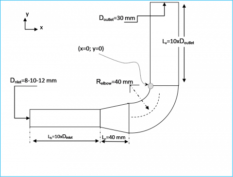
Air with pulverized olive cake particles are supplied from mixing chamber through a tube of an inner diameter 8mm, 10mm or 12mm. The burner is connected to circular elbow as shown in figure 2. The elbow is weld to conical tube of a length Lc=40 mm and the last is connected to a cylindrical tube coming from an enough long distance (Lh=10xDinlet). In addition, the vertical pipe length was chosen long enough (Lv=10xDinlet).
The discrete phase of olive cake particles have non-uniform size distribution, with diameters ranging from 0 to 200 μm. The polydisperse particle size distribution is assumed to fit the Rosin-Rammler function [11] with a mean diameter of 140 μm and a spread parameter of 3.5.
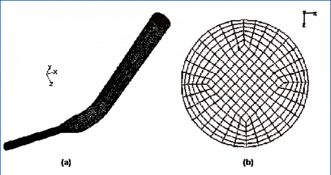
The computational domain configuration is designed by using the mesh generating software, Gambit, and is shown in Figure 3. A computational domain of a three-dimensional computational mesh was configured for use in the mixture of gas-particle flow numerical calculation. The number of cells in three configurations case 1 (Dinlet=8mm), case 2 (Dinlet =10mm) and case 3 (Dinlet =12mm) are 31860, 32040 and 59904cells respectively. Refined mesh is applied around the axis and near wall of pipe.
Simulations were performed for 5 cases which are summarized in Table 3.
Figure 2. Dimensions of pipes geometry
Figure 3. (a) Numerical grid of a pipe (example of Dinlet=10mm) and (b) Numerical grid of pipe cross-section
Table 3. Summary of simulations performed
|
Case name |
Case_1 |
Case_2 |
Case_3 |
Case_4 |
Case_5 |
|
Air flow rate,$\dot{\mathrm{m}}$f (l/s) |
2.01 |
2.01 |
2.01 |
2.01 |
2.01 |
|
Flow velocity, uf (m/s) |
15.60 |
22.46 |
35.96 |
22.46 |
22.46 |
|
Outlet diameter, Doutlet (mm) |
30 |
30 |
30 |
30 |
30 |
|
Inlet diameter, Dinlet (mm) |
12 |
10 |
08 |
10 |
10 |
|
Diameter ratio, Doutlet /Dinlet (-) |
2.50 |
3 |
3.75 |
3 |
3 |
|
Particles mean diameter,dp,mean (μm) |
140 |
140 |
140 |
120 |
190 |
|
Particles flow rate, $\dot{\mathrm{m}}$p (g/min) |
22.96 |
22.96 |
22.96 |
22.96 |
22.96 |
|
Solid loading ratio, Ø (-) |
0.15 |
0.15 |
0.15 |
0.15 |
0.15 |
5.1 Verification Simulations
To verify the validity of the calculation model and methods, simulation results and experimental data were compared. We have used the experimental data of Yilmaz and Levy [2].
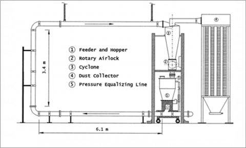
The experimental configuration represent a pneumatic conveying system consisting of two 6.1-m-long horizontal pipes and a 3.35-m-long vertical pipe as well as two 90° circular elbows. Laboratory experiments were conducted in 154 and 203 mm I.D. test sections using pulverized-coal particles (90% less than 75 mm) for two different 90° circular elbows having pipe bend radius to pipe diameter ratios of 1.5 and 3.0 (see figure 4).
Figure 4. Schematic diagram of the pneumatic conveying flow facility using by Yilmaz and Levy [2]
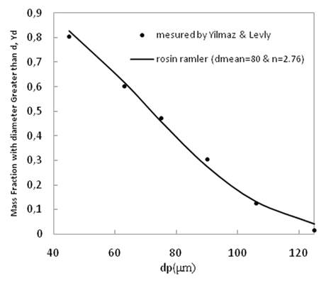
The computational flow domain of validation is limited to a horizontal pipe with a length of 10 pipe diameters, the elbow section, and a vertical pipe with a length of 20 pipe diameters. Fully developed turbulent flow was assumed at the inlet to the horizontal section [2]. A Rosin-Rammler distribution function is used to respect the measured diameter distribution with a mean diameter of 80μm and a spread parameter of 2.76 (see figure 5). Experimental measurements (see figures 6, 7 and 8) of time-average local particle concentrations were obtained using a fiber-optic probe which was traversed over the cross-section of the pipe.
Figure. 5. Rosin-Rammler Curve and Particle Size Data of Yilmaz and Levly [2]
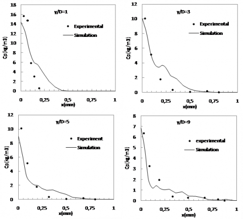
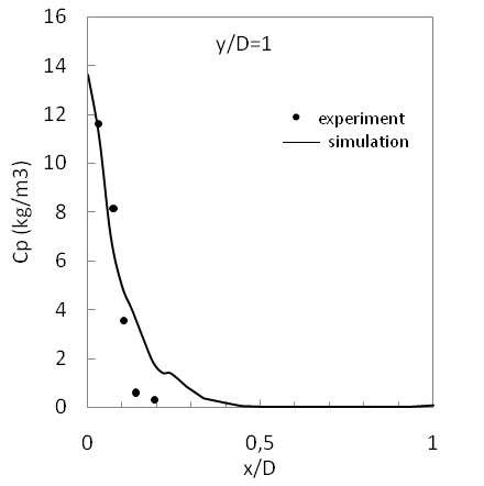
Comparison of the simulated and measured results is shown in Figures 6 and 7. The measured and computed radial profiles of the particle concentration (Cp) within elbow at different y/D axial distances are compared.
Figure 6. Comparison of CFD results and experimental data of particle concentration (Cp) profiles within elbow at different y/D distances (Relbow /D=3)
Figure 7. Comparison of CFD results and experimental data of particle concentration (Cp) profiles within elbow at different y/D distances (Relbow /D=1.5)
Figure 8. Particle mass concentration Cp (kg/m3), following elbow at y/D=3
The comparison is shown through radial direction. Although a few gaps are apparent it is evident from figures 6, 7and 8that there is a reasonable agreement between the present prediction and experimental data. The gap between data and predicted results close to the wall region is due to the improper modeling of particle–wall collision with heavy particle. In addition, the irregular particle wall interaction occurring between non-spherical particles and a rough wall is not modeled.
Although this gap, we can support the conclusion that the chosen calculation model can simulate the two phase flow of our actual pipe with particle of olive cake which are less heavy than coal particles.
In the next section, we present the dynamic behavior of the two phase flow within the pneumatic conveying system of pulverized olive cake particles.
5.2 Flow field characteristics
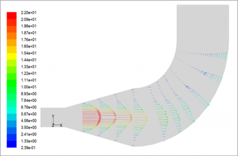
Figures 9 and 10 show the air velocity vectors and the contours of dynamics pressure for case 2, respectively.
Figure 9. Air velocity vectors (m/s): case 2
Figure 10. Contours of dynamics pressure (Pascal): case 2
In the divergent section, the flow area decrease generate of a fall in pressure near the outer wall leading to recirculation zone. A second recirculation zone takes place near the inner wall as a result of the centrifugal force in the bend section.
5.3 Effect of the inlet diameter of the pipe
Three inlet diameters of respectively 8mm, 10mm and 12mm are used, the flow rates are maintained in order to investigate the varying of the inlet diameter effect.
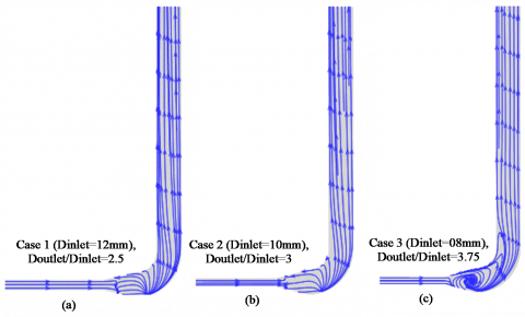
Figures 11 and 12 describe the stream lines of fluid and trajectory of particle, respectively.
Figure 11. Effect of the diameter ratio (Doutlet/Dinlet) on streamlines
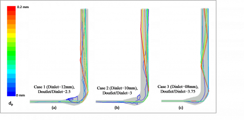
Figure 12. Examples of particles traces colored by particle diameter: Effect of the diameter ratio (Doutlet/Dinlet)
Figure 12 shows the predicted trajectories of particles in the duct. There are two types of trajectories. The first type is where the particles tend to follow the flow. This type represents the smallest diameter ones, since they possessed lower inertia and gained less momentum to overcome the drag of the fluid. The second type is where the particles don’t follow the flow and hit the outer wall bend. This type represents particles with large diameters. This can be explained as the motion of the largest particles is dominated by their inertia and hence they deviate considerably from the gas streamlines within the pipe.
The number of particle impacts in the vertical pipe increases with the decrease in the inlet pipe diameter. Indeed, particles velocity inlet varies inversely as the inlet pipe diameter (see table 3) and the inertia of particles allow these to escape from fluid turbulence and follow own trajectories.
This result is similar to one showed for aluminum oxide particles in a rectangular pipe bend; Prediction of Wadke et al [3] confirm that the number of particle impacts in the bend increases with the increase in the mean gaseous phase velocity.
Numerical results (Figures 11and 12) reveal that as the inlet diameter decrease the effect of the recirculation zone in the divergent part of the duct becomes less efficient. This can be explained as the inlet inertia of the particles becomes greater enough to overcome the drug of the fluid.
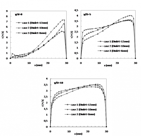
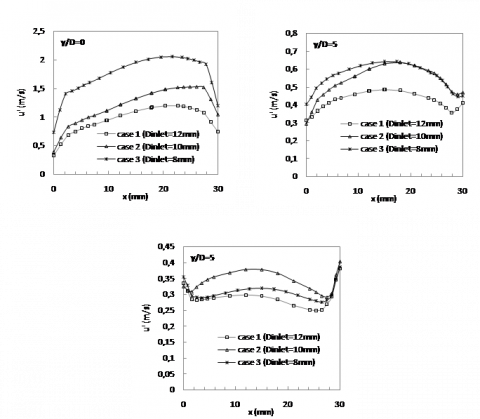
Figure 13 shows the air velocity profiles in different axial locations.
Figure 13. Effect of the diameter ratio (Doutlet/Dinlet) on the air velocity profiles along the pipe in the x direction at y/D= 0, 5, 10
From figure 13it’s easy to conclude that the maximum value of axial velocity is shifted towards the outer wall as a result of pressure gradient caused by the balance of centrifugal force and pressure gradient in the bend. As the flow advances closer to the outlet the gas flow gradually evolves towards a fully-developed turbulent structure.
Interestingly the predicted flow is sensitive to changes in the prescribed inlet conditions as the fully-developed structure is more rapidly reached in the first case (Dinlet=8mm).
Figure 14 shows a peak of rms values (u’) close to the outer wall that decrease with distance from the bend exit.
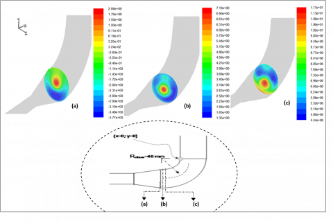
Figure 15. Effect of the diameter ratio (Doutlet/Dinlet) on particles concentration along the pipe in the x direction at y/D=0, 5, 10
Figure 15 gives the effect of diameter ratio effect on particles concentration profiles in different axial positions, it shows that a sharp peak of particles concentration occurs close to the outer wall of the duct due to the centrifugal forces created by the curvature. As the flow progress centrifugal forces and radial gradient pressure disappear. Particles gradually move to the center of the pipe.
As the inlet diameter decreases the particles inertia force become higher and the collisions between particles and the outer wall cannot be avoided and plays a role in the redistribution of particles in the air flow (figure 14).
5.4 Effect of particle size distribution
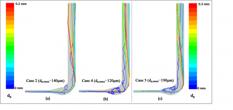
In conveying systems of pulverized combustion devices the particles diameter can vary from application to other. Particle diameter distribution influences the flow behavior since it influences the drug force. In order to investigate this effect, we have considered three cases with size distribution. Case 2 corresponds of the basic configuration and that is defined by an inlet pipe diameter of 10 mm and a mass flow rate of particles equal to 22.96 g/min. Case 4 is characterized by the lowest mean diameter of particles (dp,mean= 120 μm). Case 5 correspond of a sample of olive cake having a high mean diameter (dp,mean=190 μm) and a maximal diameter of 300 μm.
Figure 16. Examples of particles traces colored by particle diameter (Dinlet=10mm): Effect of the particle size distribution
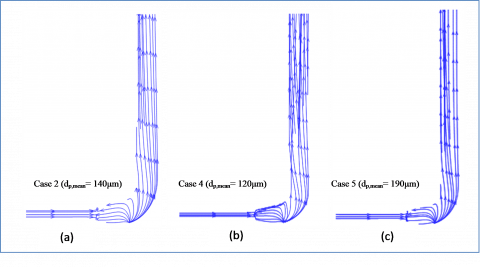
Figure 17. Effect of the particle size distribution on Streamlines
Particles of small size follow streamlines and may not impact the wall, whereas largest ones impact the outer wall as results of their high inertial speed and centrifugal force and they may rebound with enough momentum to impact the wall a second time on the inner border.
In this context, based on the different cross-sectional concentration for different particle sizes, Levy and Mason [6] have concluded that paths taken by the particles after the bend were strongly dependent upon their sizes.
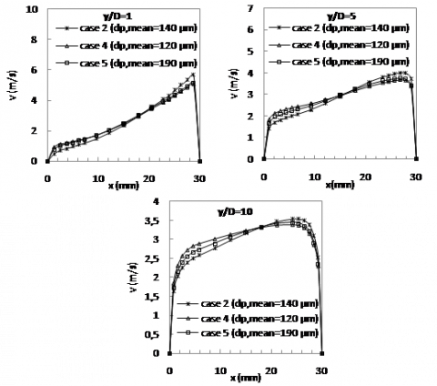
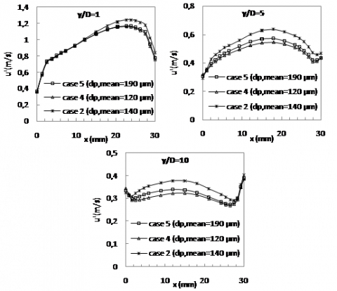
Figure 18. Effect of the particle size distribution on the fluid velocity along the pipe in the x direction at y/D= 1, 5, 10
Figures 16, 17 and 18 show that the particle concentration increases near the outer wall and decreases near the inner wall with the decrease of mean particles diameter.
Figure 19. Effect of the particle size distribution on the rms fluid velocities ($\sqrt{\frac{2}{3} \mathrm{k}}$) along the pipe in the x direction at y/D= 1, 5, 10
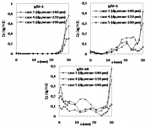
Figure 20. Effect of the particle size distribution on particles concentration along the pipe in the x direction at y/D=1, 5, 10
It can be seen from figures16, 19 and 20 that the particle-wall interaction is a main controlling factor for the outer region of the flow.
CFD calculations using Fluent 6.3 were performed to investigate the behavior of turbulent gas-solid flow a complex geometry. The effects of varying inlet/outlet diameter ratio and particles size distribution were demonstrated.
The present results help to optimize the pneumatic conveying of pulverized fuel where transitions in pipe geometry are common and the particle concentration profile can affect the combustion process.
|
CD |
Standard drag coefficient (-) |
|
Cp |
particle concentration (kg/m3) |
|
Dd |
diameter (m) |
|
e |
coefficient of restitution (-) |
|
g |
acceleration of gravity (m/s2) |
|
k |
turbulence kinetic energy (m²/s²) |
|
Le |
flow length scale (m) |
|
$\dot{\mathrm{m}}$ |
mass flow rate (kg/s) |
|
p |
pressure (Pa) |
|
R |
Pipe bend radius (m) |
|
Re |
Reynolds number (-) |
|
u |
vmean velocity (ms-1) |
|
u’ |
rms fluid velocity (ms-1) |
|
x |
Transverse distances in pipe cross-section (m) |
|
z (or y) |
Axial distance (m) |
|
Greek Letters |
|
|
Φ |
solid loading ratio (-) |
|
μ |
Fluid viscosity (kg/ms) |
|
μt |
turbulent viscosity (kg/ms) |
|
$\epsilon$ |
turbulence dissipation (m²/s3) |
|
ρ |
density (kg/m3) |
|
Subscripts |
|
|
f |
fluid |
|
c |
conical |
|
h |
horizontal |
|
n |
normal component |
|
p |
particle |
|
t |
tangential component |
|
v |
vertical |
1. D. O. Njobuenwu, M. Fairweather, Modelling of pipe bend erosion by dilute particle suspensions, Computers and Chemical Engineering 42, pp. 235– 247, 2012.
2. Yilmaz, A.; Levy, E. Formation and dispersion of ropes in pneumatic conveying. Powder Technol., 114 (1-3), pp. 168-185, 2001.
3. P. M. Wadke, M. J. Pitt, A. Kharaz, M. J. Hounslow and A. D. Salman, Particle trajectory in a pipe bend, Advanced Powder Technol., Vol. 16, No. 6, pp. 659–675, 2005.
4. L. Y. Lee, T. Y.Quek, R. Deng, M. B. Ray, Ch.H. Wang, Pneumatic transport of granular materials through a 90◦ bend, Chemical Engineering Science 59, pp. 4637 – 4651, 2004.
5. R. A. Gore, C. T. Crowe,. Effect of particle size on the modulating turbulent intensity, International Journal of Multiphase Flow, 15, 2, pp. 279-285, 1989.
6. E. Levy and D. J. Mason, The effect of bend on the particle cross-section concentration and segregation in pneumatic conveying systems, Powder Technol. 98, pp. 95–103,1998.
7. A. Aroussi, D. Giddings, E. Mozaffari and S.J. Pickering, Characterization of pulverized fuel roping, 15th International Congress of Chemical and Process Engineering (CHISA2002), Prague, Czech, 2002.
8. G. Borsuk, B. Dobrowolski and J. Wydrych, Gas-solids mixture flow through a two-bend system, Chemical and Process Engineering, 27, pp. 645-656, 2006.
9. B. Dobrowolski and J. Wydrych, Computational and experimental analysis of gas-particle flow in furnance power boiler instalations with respect to erosion phenomena, Journal of theoretical and applied mechanics, 45, 3, pp. 513-537, 2007.
10. W. A. Aissa, T.A.M. Mekhail, S.A. Hassanein and O. Hamdy, experimental and numerical study of dilute gas-solid flow inside a 90 horizontal square pipe bend, Open journal of fluid dynamics, 3, pp. 331-339, 2013.
11. User’s Guide, FLUENT 6.3, Chapter 22: Modeling Discrete Phase, section 22.12.1: Using the Rosin-Rammler Diameter Distribution Method, pp. 22-114-117, Inc, 2006.
12. E. A. Matida, K. Nishino, and K. Torii, Statistical simulation of particle deposition on the wall from turbulent dispersed pipe flow, International Journal of Heat and Fluid Flow, vol. 21, pp. 389–402, 2000.
13. M. Coppi, A. Quintino, F. salata, Fluid dynamic feasibility study of solar chimney in residentail buildings, International Journal of Heat & Technology, 29, 1, pp.1-6, 2011.
14. C. Biserni, M. De Luca, E. Lorenzini, C. Ragazzini Theoretical and numerical investigation on ship motion and propulsion in marine engineering, International Journal of Heat & Technology, 28, 2, pp. 5-9, 2010.
15. C. Yin, L. Rosendahl, S.K. Kær, T. Condra, Use of numerical modeling in design for co-firing biomass in wall-fired burners, Chemical Engineering Science 59, pp. 3281–3292, 2004.
16. S. A. Morsi and A. J. Alexander, An Investigation of Particle Trajectories in Two-Phase Flow Systems, J. Fluid Mech., 55(2), pp. 193-208, 1972.
17. J. R. Cash and A. H. Karp, A variable order Runge-Kutta method for initial value problems with rapidly varying right-hand sides, ACM Transactions on Mathematical Software, 16, pp. 201-222, 1990.
18. M. Sommerfeld, Modelling of particle-wall collisions in confined gas- particle flows, Int. J. Multiphase Flow, 18, 6, pp. 905-926, 1992.