OPEN ACCESS
Vortex-chamber is a main part of vortex tube which the pressured gas is injected into this part tangentially. An appropriate design of vortex-chamber geometry leads to better efficiency and good vortex tube performance. In this study, the computational fluid dynamics (CFD) model is created on basis of an experimental model and is a three-dimensional (3D) steady compressible model that utilizes the k-ε turbulent model. In this paper the effect of changing radius of rounding off edge at hot tube entrance (r1) on vortex tube performance has been studied for different value of r1 and the optimized radius has been determined. According to numerical results the cold temperature difference has increased when we take into account the effect of the radius of rounding off edge in the range of 0-1.5 mm and when the radius of rounding off edge has located in the range of 1.5-4 mm, the cold temperature difference has decreased. The highest ΔTc is 47.26 K for r1=1.5 mm at a cold mass fraction of 0.3, higher than basic model around 7.5% at the same cold flow fraction. Finally, the results obtained, particularly the temperature values, are compared with some available experimental data, which s how good agreement.
Numerical simulation; Vortex tube; rounding off edge radius; Pressure drop; Cooling efficiency.
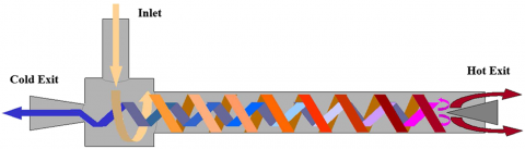
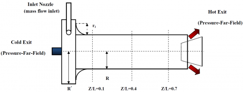
The vortex tube is a device that has a simple geometry, without any moving or complicated parts that separates a pressurized gas into hot and cold streams. A schematic drawing of a typical vortex tube and its proceeds is shown in Fig. 1. A vortex tube includes different parts such as: one or more inlet nozzles, a vortex-chamber, a cold end orifice, a control valve that is located at hot end and finally a working tube. When pressured gas is injected into the vortex-chamber tangentially via the nozzle intakes, a strong rotational flow field is created. When the gas swirls to the center of the vortex-chamber it is expanded and cooled. After occurrence of the energy separation procedure in the vortex tube the pressured inlet gas stream was separated into two different gas streams including cold and hot exit gases. The “cold exit or cold orifice” is located at near the inlet nozzle and at the other side of the working tube there is a changeable stream restriction part namely the conical control valve which determines the mass flow rate of hot exit. As seen in Fig. 1, a percent of the compressed gas escapes through the conical valve at the end of the tube as hot stream and the remaining gas returns in an inner swirl flow and leaves through the cold exit orifice. Opening the hot control valve reduces the cold air flow and closing the hot valve increases the cold mass flow rate.
Figure 1. A schematic drawing of Ranque-Hilsch vortex tube
$\alpha=\frac{\dot{m}_{c}}{\dot{m}_{i}}$ (1)
In this equation $\dot{m}_{i}$ is the mass flow rate at the cold exit and $\dot{m}_{i}$ is the inlet flow rate.
Vortex tube performance was first discovered by Ranque in 1932 [1] when he was investigating processes in a dust separation cyclone. The German physicist Rudolf Hilsch [2] improved the design of this mechanism. The detailed procedure of energy separation phenomenon is not completely understood yet. In the present investigation, instantaneous procedure of energy separation is illustrated in a vortex tube by computational data. The vortex tube has been a subject of many studies. Rafiee and Rahimi [3] performed an experimental work on convergence ratio of nozzles and in their work a three dimensional computational fluid dynamic model was introduced as a predictive tools to obtain the maximum cold temperature difference. Also they proved that energy separation procedure inside the vortex tube can be improved by using convergent nozzle. Rafiee and Sadeghiazad [4] introduced 3D CFD exergy analysis and Stephan et al. [5] proposed the constitution of Gortler vortices on the inside wall of the vortex tube that drive the fluid motion. Rafiee and Sadeghi [6] performed an experimental and numerical work on cone length of control valve of vortex tube. Skye et al [7] employed a model similar to that of Aljuwayhel. Pourmahmoud et al [8] investigated numerically the effect of convergent nozzle in flow patterns Rafiee et.al [9] numerically investigated the effect of working tube radius on vortex tube performance and the optimum working tube radius has been determined. Pourmahmoud and Rafiee [10] also performed a numerical study on working fluid importance in vortex tube applications and their study showed, CO2 is better than O2, N and air. Rahimi et al [11] conducted a numerical simulation to analysis the effect of divergent hot tubes on thermal performance of vortex tube. Pourmahmoud et al [12] and Rafiee et al [13] carried out a numerical study to understand the flow field and temperature separation phenomenon. Also some studies have been performed to use vortex tube as refrigeration device, instead of the usual refrigeration systems, for example, Alka Bani Agrawal; Vipin Shrivastava [14], and Jayaraman, Senthil Kumar [15]. Volkan Kirmaci [16] used Taguchi method to optimize and simulate the number of nozzles of vortex tube. In general definition, exergy is the maximal work, attainable in given source state with any generalized friction. In closed system energy is conserved but exergy is destroyed due to generalized friction. In the thermodynamics the exergy of a system is a maximum useful work possible during a procedure that brings the system into balance with a heat reservoir. The units of exergy are the same as for energy or heat, such as kilocalories, joules, BTUs, etc. Some of the exergy investigations are briefly mentioned below. Rafiee et al [17] carried out an experimental study about characteristic analysis of the performance of a counter flow Ranque-Hilsch vortex tube with regard to control valve angle. Ceylan et al [18] performed an exergy research for timber dryer assisted heat pump. Kirmaci [19] carried out exergy analysis of a counter flow RanqueHilsch vortex tube with different nozzle numbers at various inlet pressures. This study was performed using O and air as pressured inlet gas. Also in other fields some works have been done, for example, Ozgener and Hepbasli [20], Saidur et al [21], Esen et al [22]. A valuable work was done to analyze the isotope separation using vortex tubes by Lorenzini et al. [23].
In the presented work with assuming the advantages of using different radius of rounding off edge on the energy separation process and its considerable role on the creation of maximum cooling capacity of machine, the optimum radius is elected. This research believes that choosing an appropriate design of vortex-chamber is the one of important physical parameters for obtaining the highest refrigeration efficiency. So far numerical investigations towards optimization of rounding off edge radius has not been done but the importance of this object can be regarded as an interesting theme of research so that the machine would operate in the way that maximum cooling effect or maximum refrigeration capacity is provided.
The compressible turbulent and highly rotating flow inside the vortex tube is assumed to be three-dimensional, steady state and employs the standard k-ε turbulence model on basis of finite volume method. The RNG k-ε turbulence model and more advanced turbulence models such as the Reynolds stress equations were also investigated, but these models could not be converged for this simulation (Rafiee et al. [3]). Rafiee et al. [6] showed, for this reason that the numerical results has good agreement with the experimental data, the k-ε model can be selected to simulate the effect of turbulence inside the computational domain. Consequently, the governing equations are arranged by the conservation of mass, momentum and energy equations, which are given by:
The equation for conservation of mass, or continuity equation, can be indicated as follows:
$\frac{\partial \rho}{\partial t}+\nabla \cdot(\rho \vec{v})=S_{m}$ (2)
The flow field in this investigation has been assumed ‘steady state’ and term Sm is the mass added to continuous domain from other domains.
Momentum equation:
$\frac{\partial}{\partial x_{j}}\left(\rho u_{i} u_{j}\right)=-\frac{\partial p}{\partial x_{i}}+\frac{\partial}{\partial x_{j}}\left[\mu\left(\frac{\partial u_{i}}{\partial x_{j}}+\frac{\partial u_{j}}{\partial x_{i}}-\frac{2}{3} \delta_{i j} \frac{\partial u_{k}}{\partial x_{k}}\right)\right]+\frac{\partial}{\partial x_{j}}(-\overline{\rho u_{i}^{\prime} u_{j}^{\prime}})$ (3)
Energy equation:
$\frac{\partial}{\partial x_{i}}\left[u_{i} \rho\left(h+\frac{1}{2} u_{j} u_{j}\right)\right]=\frac{\partial}{\partial x_{j}}\left[k_{e f f} \frac{\partial T}{\partial x_{j}}+u_{i}\left(\tau_{i j}\right)_{e f f}\right]$
$k_{e f f}=K+\frac{c_{p} \mu_{t}}{\operatorname{Pr}_{t}}$ (4)
Since we determined the working fluid is an ideal gas, then the compressibility effect must be considered as below:
$p=\rho R T$ (5)
The turbulence kinetic energy (k) and the rate of dissipation (ε) are obtained from the following equations:
$\frac{\partial}{\partial t}(\rho k)+\frac{\partial}{\partial x_{i}}\left(\rho k u_{i}\right)=\frac{\partial}{\partial x_{j}}\left[\left(\mu+\frac{\mu_{t}}{\sigma_{k}}\right) \frac{\partial k}{\partial x_{j}}\right]+G_{k}+G_{b}-\rho \varepsilon-Y_{M}$ (6)
$\frac{\partial}{\partial t}(\rho \varepsilon)+\frac{\partial}{\partial x_{i}}\left(\rho \varepsilon u_{i}\right)=\frac{\partial}{\partial x_{j}}\left[\left(\mu+\frac{\mu_{t}}{\sigma_{\varepsilon}}\right) \frac{\partial \varepsilon}{\partial x_{j}}\right]+C_{1 \varepsilon} \frac{\varepsilon}{k}\left(G_{k}+C_{3} G_{b}\right)-C_{2 \varepsilon} \rho \frac{\varepsilon^{2}}{k}$ (7)
In these equations, Gk, Gb, and YM represent the generation of turbulence kinetic energy due to the mean velocity gradients, the generation of turbulence kinetic energy due to buoyancy and the contribution of the fluctuating dilatation in compressible turbulence to the overall dissipation rate, respectively. C1ε and C2ε are constants. σk and σε are the turbulent Prandtl numbers for k and ε also. The turbulent (or eddy) viscosity, µt , is computed as follows:
$\mu_{t}=\rho C_{\mu} \frac{k^{2}}{\varepsilon}$ (8)
Where, Cμ is a constant. The model constants C1ε, C2ε, Cμ, σk and σε have the following default values: C1ε = 1.44, C2ε = 1.92, Cμ = 0.09, σk = 1.0, σε = 1.3.
3.1 3D CFD MODEL
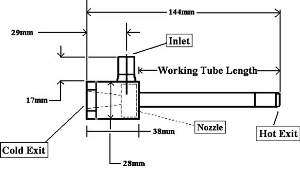
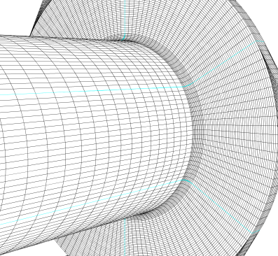
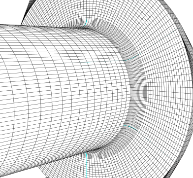
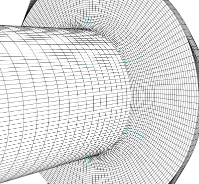
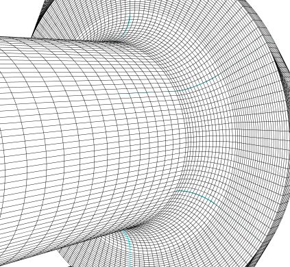
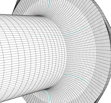
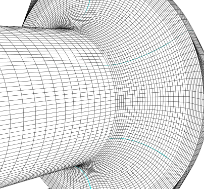
The 3D CFD model is created on basis of that was used by Skye et al. [7] in their experimental (Fig. 2) work. It is noteworthy that, an ExairTM 708 slpm [16] vortex tube was used by Skye et al. [7] to perform all tests and to take all of the experimental data. The dimensional geometry of this vortex tube has been summarized in the Tab. 1. The 3D CFD mesh grid is shown in Fig. 4. In this model a regular organized mesh grid has been used. All radial line of this model of meshing has been connected to the centerline and the circuit lines have been designed organized from wall to centerline. So, the volume units that have been created in this model are regular cubic volumes. This meshing system helps the computations to be operated faster than the irregular and unorganized meshing, and the procedure of computations have been done more precisely.
Figure 2. Schematic of vortex tube that used by Skye et al
Table 1. Geometric measurements of the vortex tube that was used by Skye et al. (2006)
|
Measurement |
Value |
|
Working tube length |
106 mm |
|
Nozzle height |
0.97 mm |
|
Nozzle width |
1.41 mm |
|
Nozzle total inlet area (An) |
8.2 mm2 |
|
Cold exit diameter |
6.2 mm |
|
Cold exit area |
30.3 mm2 |
|
Hot exit diameter |
11 mm |
|
Hot exit area |
95 mm2 |
For this reason the CFD model has been assumed a rotational periodic condition. Hence, only a sector of the flow domain with angle of 60° needs to consider for computations as shown in Fig. 3.
r1=0.5 mm
r1=1mm
r1=1.5mm
r1=2mm
r1=3mm
r1=4mm
Figure 3. Different rounding of edges at hot tube entrance
3.2. BOUNDARY CONDITIONS
Boundary conditions for this study have been indicated in Fig. 4. The inlet is modeled as mass-flow-inlet .The inlet stagnation temperature and the total mass flow inlet are fixed to 294.2 K and 8.35 g s-1 respectively according to experimental conditions. A no-slip boundary condition is used on all walls of the system. For the cold and hot exits, two kinds of boundary condition can be used for numerical analysis. The first boundary condition is pressure-outlet and the second one can be considered as pressure-far-field. The pressure-outlet boundary condition is used when the outlet pressures on both cold and hot outlets are known. However, the pressure-far-field boundary condition is used for the models with unknown outlet pressures.
Figure 4. A schematic form of boundary conditions
In this article both kinds of these boundary conditions are used for cold and hot exits. For pressure-outlet boundary condition, the static pressure at the cold exit boundary was fixed at experimental measurements pressure and the static pressure at the hot exit boundary is adjusted in the way to vary the cold mass fraction. The pressure-far-field boundary condition which is also employed for both exhausts including hot and cold exit is a state when the static pressures at the exhausts of vortex tube are not determined exactly. In the other hand, a vortex tube usually works in the ambient condition and for change in the cold mass fraction one need to change the area of hot exit that is the true action for this purpose in comparison with pressure-outlet boundary condition. In this article, both kinds of boundary conditions are applied and investigated numerically and the results compare to each other. The computations in this study utilize a pressure correction based iterative SIMPLE algorithm for discretising the convective transport terms. A compressible form of the Navier-Stokes equation along with the standard k-ε model by second order upwind for momentum, turbulence and energy equations has been used to simulate the phenomenon of flow pattern and temperature separation in a vortex tube with 6 straight inlet nozzles operating under condition of using different geometry of vortex-chamber by using the FLUENTTM software package. The default values of under-relaxation factor are shown in Table 2.
Table 2. Under-relaxation factors used for computations
|
Under-Relaxation Factor |
Value |
|
Pressure |
0.3 |
|
Density |
1 |
|
Body Force |
1 |
|
Momentum |
0.7 |
|
Turbulent Kinetic Energy |
0.8 |
|
Turbulent Dissipation Rate |
0.8 |
|
Turbulent Viscosity |
1 |
|
Energy |
1 |
The numerical results obtained from the models, which involve the effect of rounding off edge radius change on different vortex tube thermo and physical characteristics, are presented in this section.
4.1 Validation
The previous CFD researches on vortex tube usually have been performed in the fixed boundary condition such as pressure at the hot and cold exits. These values of pressure at exhausts are taken from experimental process that has been achieved during the experiment procedure. Since these pressures are not available always, this paper utilizes a useful method with any necessity of pressure values at cold and hot exit. This method is useful and suitable for CFD researchers that are involved in vortex tube fields. In this method, the pressure values of exhausts in the vortex tube are not necessary to be available and the prediction is independent of pressure values at the exhausts. In this paper and this method the pressure boundary condition adjusted as pressure-far-field condition. This means that the vortex tube is working in ambient conditions. In order to achieve the certain cold mass fraction, we have to change the area of hot exhaust. In the real state (Experimental) changing the hot exit area is achieved by the action of hot control valve.
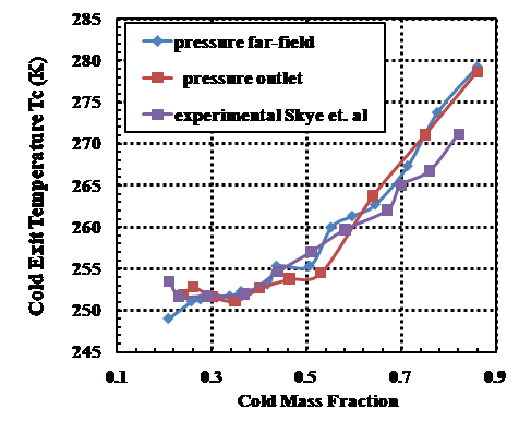
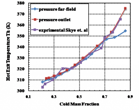
In this section, the both kinds of boundary conditions for exhaust i.e. pressure-far-field boundary condition and pressure-outlet boundary condition are applied to the CFD model together with other boundary conditions for inlet, wall and periodic planes which described in section 3.2 and cold and hot exit temperatures are derived and compared with experimental data to demonstrate that there is not noticeable difference for these two kinds of boundary conditions. As seen in Fig. 5 and 6, cold and hot exit temperatures for both boundary conditions as a function of cold mass fraction (α) have good agreement with the experimental data. The presented data in Fig. 5 and 6 are the minimum and maximum temperature achieved for cold and hot exits respectively. In Fig. 5 the minimum Tc =250.24 K and Tc= 249.6 K is obtained at about $\alpha$=0.3 through the CFD simulations and experiments respectively. The maximum and minimum difference between CFD results and experimental data in cold temperatures is about 3.32% and 0.18% respectively. This difference for hot temperature at the peak of its value reaches to 3.77%. As seen in Fig. 6, the applied 3D CFD model can produce maximum hot gas temperature of 354.34 K at $\alpha$=0.86 and a minimum cold gas temperature of 250.24 K at about 0.3 cold mass fraction. It should be mentioned that the validation part has been done for compressed air as operation fluid.
Figure 5. Comparison of cold exit temperature for both kinds of exhausts boundary conditions with the experimental data
Figure 6. Comparison of hot exit temperature for both kinds of exhausts boundary conditions with the experimental data
4.2 Grid independence study
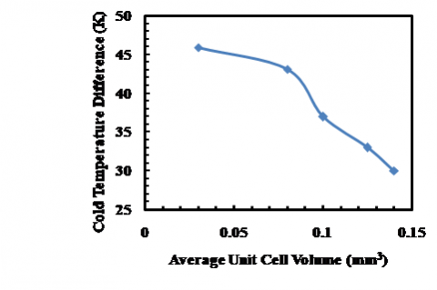
The 3D CFD analysis has been performed for different average unit cell volumes in vortex tube as a computational domain. This is for the reason that removing probable errors arising due to grid coarseness. Therefore, first the grid independence study has been done for $\alpha$=0.3. As seen in the Fig. 5, at this cold mass fraction the vortex tube (with 6 straight nozzles) achieves a minimum outlet cold gas temperature. Consequently, in the most of the evaluations we use $\alpha$=0.3 as a special value of cold mass fraction.
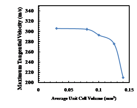
The variation of cold exit temperature difference and maximum tangential velocity as the main parameters are shown in Figs. 7 and 8 respectively for different unit cell volumes. Not much major advantage can be seen in reducing of the unit cell volume size below 0.026 mm3; which corresponds to 287000 cells.
Figure 7. Grid size independence study on cold temperature difference at different average unit cell volume
Figure 8. Grid size independence study on maximum swirl velocity at different average unit cell volume
4.3 An investigation into the optimization of R*
In this section the effect of changing radius of vortex-chamber (R*) on vortex tube performance has been studied for seven different values (R*= 5.7, 6.4, 7, 9, 11, 12 and 13) of R*. For each of these models, a 3D CFD model has been created and the results of computations in these models have been compared with each other. The compared results are: tangential velocity, total temperature and total pressure. The total temperature separation results for the seven cases are provided in Tab. 3, below:
Table 3. Total temperature separation at cold mass fraction α = 0.3 in the CFD models
|
Model |
R* (mm) |
Tc(K) |
Th(K) |
∆Tc (K) |
∆Th (K) |
∆Tt (K) |
|
Case (a) |
5.7 |
250.2 |
311.5 |
43.96 |
17.3 |
61.26 |
|
Case (b) |
6.4 |
249.3 |
311.7 |
44.81 |
17.5 |
62.36 |
|
Case (c) |
7 |
249.3 |
312.7 |
44.9 |
18.5 |
63.47 |
|
Case (e) |
9 |
247.6 |
313.4 |
46.55 |
19.2 |
65.8 |
|
Case (g) |
11 |
247.4 |
313.3 |
46.77 |
19.1 |
65.95 |
|
Case (h) |
12 |
248.1 |
313.7 |
46.1 |
19.5 |
65.61 |
|
Case (i) |
13 |
248.4 |
313.5 |
45.77 |
19.3 |
65.16 |
As Table 3, this is clearly observable that the cold temperature difference magnitude in the model of R*=11 mm [Case (g)] is the greatest value among the all of created models.
4.4 An investigation into the optimization of r1
In this section the effect of rounding off edge radius variations at tube’s entrance inside the vortex-chamber on vortex tube performance has been studied for thirteen different values (r1= 0, 0.25, 0.4, 0.5, 0.75, 1, 1.25, 1.5, 1.75, 2, 2.5, 3 and 4mm) of r1. For each of these models, a 3D CFD model has been created and the results of computations in these models have been analyzed. The compared results are: Total temperature and total pressure. The total temperature separation results for seven cases are presented in Tab. 4, below:
Table 4. Total temperature separation at cold mass fraction α = 0.3 in the CFD models
|
Model |
r1 (mm) |
Tc (K) |
Th (K) |
∆Tc (K) |
∆Th (K) |
∆Tt (K) |
|
Case (g) |
0 |
247.4 |
313.3 |
46.77 |
19.1 |
65.9 |
|
Case (q) |
0.5 |
247.2 |
313.9 |
46.92 |
19.7 |
66.6 |
|
Case (m) |
1 |
246.9 |
313.5 |
47.23 |
19.3 |
66.5 |
|
Case (n) |
1.5 |
246.9 |
313.5 |
47.26 |
19.3 |
66.6 |
|
Case (o) |
2 |
247.0 |
313.4 |
47.2 |
19.2 |
66.4 |
|
Case (p) |
3 |
247.1 |
313.3 |
47.03 |
19.1 |
66.1 |
|
Case (k) |
4 |
247.5 |
313.2 |
46.7 |
19.0 |
65.7 |
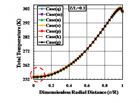
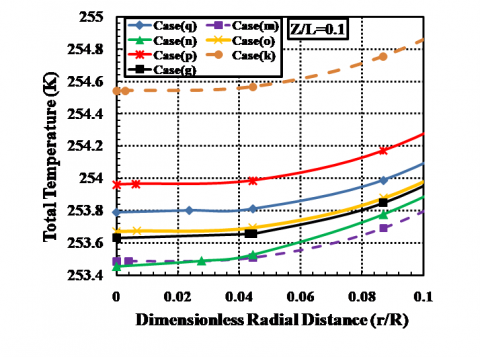
Total temperature and total pressure. In order to illustrate the effect of variation of rounding off edge radius at tube’s entrance inside the vortex-chamber on radial profiles of total temperature and total pressure, the profiles at two axial locations (Z/L= 0.1and 0.7) at the cold mass fraction 0.3 as a function of dimensionless radial distance were studied, the diagrams of which are depicted in Figs. 9, 10 and 11.
(a)
(b)
Figure 9. a) Radial profile of total temperature at Z/L=0.1 for ε =0.3. b) The marked area on Fig.9.a
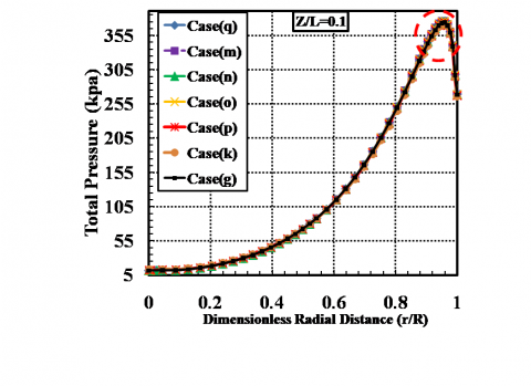
As seen in Fig. 9, the minimum total temperature near the cold exit (Z/L=0.1) is occurred with case (n) and is about 253.42 K. The ΔTc increases with the increase of r1 up to about r1 = 1.5 mm and reaches the maximum value. Thereafter cold temperature difference decreases with the further increase of r1. In Fig. 9, it can be seen that, the value of r1 should be neither too large nor too small and r1 = 1.5mm is the best candidate to achieve the highest ΔTc. Figure 10 and 11 illustrate the total pressure variations for different radiuses of rounding off edge at the two axial locations Z/L= 0.1 and 0.7 as a function of dimensionless radial distance of working tube.
(a)
(b)
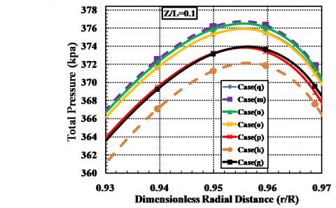
Figure 10. a) Radial profile of total pressure at Z/L=0.1 for α =0.3.b) The marked area on Fig.10.a
Optimization by simulation of r1 variations leads to an improvement in total pressure at Z/L=0.1, eventually it reaches 376.4 kpa.
(a)
(b)
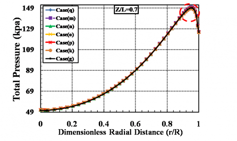
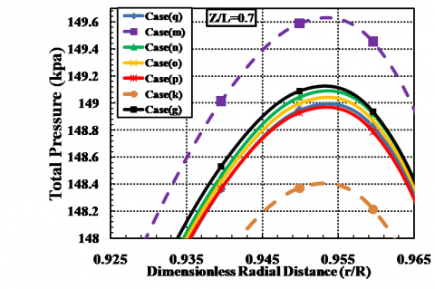
Figure 11. a) Radial profile of total pressure at Z/L=0.7 for α =0.3.b) The marked area on Fig.11.a
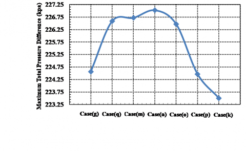
As seen in Fig. 10 and 11, fluid stream has greater total pressure in case (m) in comparison with other cases. Maximum total pressure difference between Z/L=0.1 and Z/L=0.7 can be observed in Fig. 12 and according to this Figure, case (n) has the greatest value of pressure drop across the working tube among the all of presented models. This value of pressure drop shows an appropriate energy separation procedure in this model.
Figure 12. Maximum total pressure drop between Z/L=0.1 and Z/L=0.7
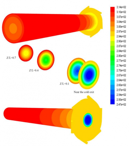
The contours of total temperature of optimum model for the inlet gas temperature 294.2 K and cold mass fraction 0.3 are shown in Fig. 13.
This paper presents the results of a series of numerical simulations focusing on various geometries of the ‘‘vortex-chamber” for constant inlet mass flow rate and cold mass fraction. Specifically, the models were conducted using different rounding off edge radiuses at tube’s entrance inside the vortex-chamber. In the present research, a 3D CFD model was used for applying as a predictive tool in the investigation of a vortex tube performance. The most important purpose of this study and optimization is the increasing total pressure and tangential velocity at the junction of vortex-chamber and working tube furthermore creation of the maximum pressure drop and velocity drop across the working tube which is shown in the pressure and velocity Figures. These conditions is the most important sign of appropriate energy separation procedure inside the vortex tube which leads to improvement of cold temperature difference and better cooling capacity. The 3D computational fluid dynamics model used in this study is a steady model that employs standard k-ε turbulence model to perform the computation procedure of results. In this investigation, the numerical results have been obtained for a counter flow Ranque-Hilsch vortex tube having r1= 0, 0.25, 0.4, 0.5, 0.75, 1, 1.25, 1.5, 1.75, 2, 2.5, 3 and 4mm; L/D=9.298 when used with air as system fluid. These models were tested and thermal performance has been realized. Cold mass fraction was fixed at α =0.3. The results present that there is the optimum value of r1 for obtaining the highest refrigeration efficiency, and 1.5mm rounding off edge radius is the optimal candidates under our computational conditions. According to numerical results the total temperature difference has increased when we take into account the effect of the rounding off edge radius in range of 0-1.5 mm and when the radius of rounding off edge has located in range of 1.5- 4 mm; the total temperature difference has decreased. It has been seen that the maximum total temperature difference is achieved when r1=1.5mm [case (n)] among the twelve primitive CFD models. It has also been seen the pressure and velocity drop has maximum value in this model. The highest ΔTc is 47.26 K for r1=1.5mm at a cold mass fraction of 0.3, higher than basic model around 7.5% at the same cold flow fraction.
Figure 13. Contours of total temperature of the optimum model at Ti= 294.2 K
1. G.J. Ranque, Experiments on expansion in a vortex with simultaneous exhaust of hot air and cold air, Le J. de Physique et le Radium. 4 (1933) 112-114.
2. R. Hilsch, The use of expansion of gases in a centrifugal field as a cooling process, Rev. Sci. Instrum. 18 (1947) 108-113.
3. S. E. Rafiee and M. Rahimi, Experimental study and three dimensional (3D) computational fluid dynamics (CFD) analysis on the effect of the convergence ratio, pressure inlet and number of nozzle intake on vortex tube performance-Validation and CFD optimization, Energy, vol. 63, pp. 195204, 2013.
4. Rafiee, S.E and Sadeghiazad, M.M, 3D cfd exergy analysis of the performance of a counter flow vortex tube , International Journal of Heat and Technology, Volume 32, Issue 1-2, 2014, Pages 71-77.
5. K. Stephan, S. Lin, M. Durst, F. Huang, D. Seher, An investigation of energy separation in a vortex tube, Int. J. Heat Mass Transfer, vol. 26, pp. 341-348, 1983.
6. S. E. Rafiee, M. M. Sadeghiazad, Three-dimensional and Experimental investigation on the effect of cone length of throttle valve on thermal performance of a vortex tube using k-ɛ turbulence model, Applied Thermal Engineering, vol. 66, pp. 65-74, 2014.
7. H. M. Skye, G. F. Nellis, S. A. Klein, Comparison of CFD analysis to empirical data in a commercial vortex tube, Int. J. Refrig, vol. 29, pp. 71-80, 2006.
8. N. Pourmahmoud, A. Hassanzadeh, S. E. Rafiee, M. Rahimi, Three Dimensional Numerical Investigation of Effect of Convergent Nozzles on the Energy Separation in a Vortex Tube, International Journal of Heat and Technology, vol. 30(2), pp. 133-140, 2012.
9. S. E. Rafiee, M. Rahimi, N. Pourmahmoud, Three dimensional numerical investigation on a commercial vortex tube based on an experimental model- Part Ӏ: Optimization of the working tube radius, International Journal of Heat and Technology, vol. 31(1), pp. 49-56, 2013.
10. N. Pourmahmoud, S. E. Rafiee, M. Rahimi, A. Hasanzadeh, Numerical energy separation analysis on the commercial Ranque-Hilsch vortex tube on basis of application of different gases, Scientia Iranica, vol. 20(5), pp. 1528-1537, 2013.
11. Rahimi, M., Rafiee, S.E., Pourmahmoud, N. Numerical investigation of the effect of divergent hot tube on the energy separation in a vortex tube, International Journal of Heat and Technology, 2013, Volume 31, Issue 2, 2013, Pages 17-26.
12. N. Pourmahmoud., M. Rahimi., S. E. Rafiee., A. Hassanzadeh, A NUMERICAL SIMULATION OF THE EFFECT OF INLET GAS TEMPERATURE ON THE ENERGY SEPARATION IN A VORTEX TUBE, Journal of Engineering Science and Technology, Vol. 9, No. 1 (2014) page 81 - 96.
13. S. E. Rafiee and M. Rahimi, Three-Dimensional Simulation of Fluid Flow and Energy Separation inside a Vortex Tube, Journal of Thermophysics and Heat Transfer, 2014, Vol.28: page 87-99, 10.2514/1.T4198.
14. A. B. Agrawal, V. Shrivastava, Retrofitting of vapour compression refrigeration trainer by an eco-friendly refrigerant, Indian J. Sci. Technol, vol. 3(4), 2010.
15. B. Jayaraman, P. Senthil Kumar. Design, optimization and performance analysis of orifice pulse tube cryogenic refrigerators. Indian J. Sci. Technol, vol. 3(4), 2010.
16. V. Kirmaci, Optimization of counter flow Ranque- Hilsch vortex tube performance using Taguchi method. International Journal of Refrigeration, vol. 32, pp. 1487-1494, 2009.
17. Seyed Ehsan Rafiee, M. M. Sadeghiazad, Effect of Conical Valve Angle on Cold-Exit Temperature of Vortex Tube, Journal of Thermophysics and Heat Transfer, 2014, Vol.28: page 785-794, 10.2514/1.T4376.
18. I. Ceylan, M. Aktas, H. Dogan, Energy and exergy analysis of timber dryer assisted heat pump, Applied Thermal Engineering, vol. 27, pp. 216-222, 2007.
19. V. Kirmaci, Exergy analysis and performance of a counter flow Ranque-Hilsch vortex tube having various nozzle numbers at different inlet pressures of oxygen and air. International Journal of Refrigeration, vol. 32, pp. 16261633, 2009.
20. O. Ozgener, A. Hepbasli, A review on the energy and exergy analysis of solar assisted heat pump systems, Renewable and Sustainable Energy Reviews, vol. 11, pp. 482-496, 2007.
21. R. Saidur, M.A. Sattar, H.H. Masjuki, H. Abdessalam, B.
S. Shahruan, Energy and exergy analysis at the utility and commercial sectors of Malaysia, Energy Policy, vol. 35, pp. 1956-1966, 2007.
22. H. Esen, M. Inalli, M. Esen, K. Pihtili, Energy and exergy analysis of a ground-coupled heat pump system with two horizontal ground heat exchangers, Building and Environment, vol. 42, pp. 3606-3615, 2007.
23. E.Lorenzini, M.Spiga, Aspetti fluidodinamici della separazione isotopica mediante tubi a vortice di Hilsch Ingegneria, n. 5-6, pp. 121-126 (maggio-giugno 1982).