Vladimir Krivtsov* | Irene Pluchinotta | Alessandro Pagano
© 2023 IIETA. This article is published by IIETA and is licensed under the CC BY 4.0 license (http://creativecommons.org/licenses/by/4.0/).
OPEN ACCESS
Systems Thinking and adequate modelling skills related to System Dynamics (SD) are essential for sustainable functioning of human society. The process of learning these skills can be considerably facilitated through hands-on experience with modern interactive tools in a play-like activity. Here we present a concise hands-on course on SD Modelling and Systems Thinking, give a brief description of its teaching materials (available online for free download), and discuss its potential developments, overall relevance and further implications. The course contains a session on ‘Systems Thinking’, and two hands-on sessions aiming to provide basic and more advanced modelling skills. Central to the latter are the examples of structural modifications for the Ebbsfleet Garden City water management model. The model represents complex processes associated with a multitude of interconnected social, technical and environmental issues. This publication provides both an important update of this model incorporating a dimensional analysis and the hands-on teaching support designed to aid knowledge transfer. It is envisaged that, with modifications, this freely downloadable course could be of use for modules related to a wide range of fundamental and applied disciplines, including e.g., Ecology, Geography, Engineering, Social and Environmental Sciences. It is expected that University students and other users will not only benefit from enhancing their understanding of the complexity of the specific problems considered by the examples used, but will also gain valuable basic system modelling skills through ‘learning by doing’. The teaching materials presented here may be particularly useful for environmental projects involving participatory approaches.
active learning, blue-green cities, complex interactions, ecological patterns, emergent behaviour, industrial ecosystem, nature-based solutions, parameter space
System Dynamics (SD) is a simulation-based methodology, combining Systems Thinking with dynamic simulation. SD provides meaningful understandings of real-world complex problems [1]. SD was originally introduced by Forrester [2] as a modelling technique for assisting corporations in understanding the long-term impact of management policies. Since then, the SD modelling approach has been extensively applied to many problems in social, economic, technological and ecological systems. In practice, SD has proven to be a very powerful tool for analysing the non-linear behaviour of systems over time [1]. For instance, Forrester [3] utilized the SD approach to capture the life cycle dynamics of urban growth and decay, considering the city environment as a complex system that undergoes drastic changes over time. Another well-known example of SD application outside the business environment is the worldwide bestseller The Limits to Growth [4], in which a team of researchers studied what could happen to the global population and to the environment if development is sustained by uncontrolled use of resources. SD modelling is also widely used for analysis of natural and industrial ecosystems [5-11]. In ecology, SD helped to derive the fundamental rule for regulation of consecutive successional stages [12] and an innovative method to control eutrophication [13, 14].
Although mathematical modelling is ubiquitously used in most branches of modern science, good SD modelling skills are in relatively short supply. On one hand, the lack of easily accessible resources for introductory learning (e.g., Skaza et al. [15] report on barriers and needs) and, on the other hand, the unfeasibility for the average audience to attend a year or term long SD course (e.g., Fisher [16] reflects on teaching a long SD course), could represent some of the limits. Acquisition of these skills is inseparably linked with the process of learning Systems Thinking and may be greatly aided through a short and hands-on experience with interactive tools in a play-like activity. Here we present a concise introductory course on SD modelling and Systems Thinking, give a brief description of its teaching materials (available online for free download), and discuss their potential development, overall relevance and wider implications. The development of the course and publication of this paper aim to address the gap between the demand for modelling skills related to Systems Thinking and SD, and the fact that those skills are in relatively short supply.
The course presented here contains a session on ‘Systems Thinking’, and two hands-on sessions aiming to provide basic (Session 1, covering a simple population model) and more advanced (Session 2, covering Ebbsfleet Garden City water management model [17]) modelling skills. Central to the latter are the examples of structural modifications for the Ebbsfleet model previously described in detail in the conference paper published in WIT transactions [18]. The model represents complex processes associated with a multitude of interconnected social, technical and environmental issues related to water management. This publication provides an important update of this existing model with the freely and easily downloadable code immediately available for further developments and applications by other users, and the hands-on teaching methodology designed to aid knowledge transfer and facilitate the learning process.
SD modellers seek to analyse complex problems by representing important system structures (including feedbacks, accumulations, delays, nonlinearities, etc.) using mathematical equations. As described in Ref. [1], an SD model (SDM) describes a system through the use of feedback loops, stocks and flows. Stocks characterize the state of the system, and keep memory of it, enabling to monitor its status. Flows affect the stocks via inflow or outflow and interlink the stocks within a system. Feedback loops are key structures in SDM and can describe mechanisms that tend to amplify whatever is happening in the system, or that counteract and oppose change, describing self-correcting processes that seek balance and equilibrium [19]. SD modelling approach is both qualitative/conceptual and quantitative/numerical. Qualitative modelling (Causal Loop Diagrams, CLDs) can greatly improve the conceptual system understanding.
As stated by Sterman [19] [1, page 137], CLDs ‘are an important tool for representing the feedback structure of systems. They are used to represent the causal connections between elements of the system in a static way. CLDs are also used to visualise mental models, which are an internal conceptual representation of an external dynamic system (historical, existing, or projected). The internal representation is analogous to the external system and contains, at a conceptual level, variables, causal links, reinforcing and balancing feedback loops, that in a simulation model are then transformed into causally-linked stocks, flows and/or other intermediary variables [20].
CLDs help to structure messy problems by combining theories and knowledge about causality, to formulate dynamic hypothesis of the behaviour of a system, identify feedback loops and elicit potential unintended consequences. Construction of a CLD is a standalone qualitative modelling approach. Often, however, it is also the starting point for quantitative SDMs.
On the other hand, quantitative SD modelling (stock-and-flow models), allows researchers to investigate and visualise dynamic hypotheses and simulate their consequences, relative to a reference (e.g., business-as-usual) scenario, so making it possible to evaluate the risks and benefits of alternative system interventions. It is useful to mix different sources of information and datasets, combining vernacular and scientific data. Sessions 1 and 2 of the course described here focus on quantitative modelling using a model of water management in Ebbsfleet Garden City developed previously [17] and its subsequent modifications [18].
Sometimes variables which correspond to stocks are designated by rectangles (without flows) in hybrid diagrams, capturing both the static causal relationships of the CLD and the dynamisms of the stock and flow simulation model. For supporting readability of the figures, this paper does not use the hybrid diagrams.
The development of a CLD and of a stock and flow model can both be achieved through a participatory approach. The outcome of this process is a participatory SDM whose development is facilitated by Group Model Building - see e.g. [21] and references therein. The Ebbsfleet city model is an example of such a participatory SDM, as it was built and validated in sessions with stakeholders and problem owners. Participatory SDMs help building a shared mental model, facilitating learning and creating a sense of ownership of the model among stakeholders. The participatory approach increases chances of adoption and implementation of model results. The phases of the Ebbsfleet city SDM (used as an example model in our teaching materials - see description of Session 2 below) are described in Ref. [17].
SD modelling is facilitated by Systems Thinking. The process of Systems Thinking represents a holistic notion, and it can be subdivided into the following steps [1]:
This paper presents a short hands-on course aiming to address the gap between the demand and the availability of modelling skills related to Systems Thinking and SD. All the teaching materials described below are freely available to download. This course has the following objectives:
The course consists of two core practical sessions on quantitative modelling and a session on qualitative modelling. All the course materials (including step-by-step instructions and descriptions of the activities for specific sessions) are available for download in the supplementary materials for this paper [https://www.researchgate.net/publication/365345624_EbbsfleetSDMtutorialBundleNov2022].
Session on systems thinking
This tutorial session is designed to give the learners basic skills and knowledge on how to apply Systems Thinking and create a qualitative model. The session consists of two parts, and can be used either as a standalone session, an additional session of the course, or as a source of reference materials (e.g., Part A is most relevant for Session 1, Part B for Session 2). The recommended time to complete this session is 1.5 hrs. It is suitable for either classroom or online delivery, or for self-study. The recommended preliminary reading for this session is the study on [1] and many more helpful sources can be found on the web. It is expected that by the end of this session the learners should be able to understand the fundamental principles of CLDs.
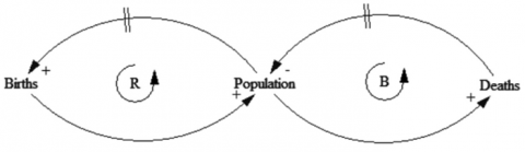
Part A introduces the typical components of a CLD [1] using an example of a simple population model (Figure 1):
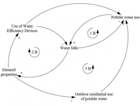
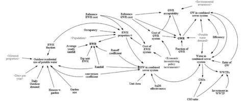
Part B uses the published example of a larger model describing the use of Potable Water in Ebbsfleet [17]. Using the information provided, learners are encouraged to gradually familiarise themselves with the Ebbsfleet city CLD and try to answer a number of relevant questions (see Figure 2 and Table 1). This gradual introduction of the materials facilitates the comprehension of the CLD structure and its building process, and prepares the learners for subsequent use of the SDM of the urban water management in Ebbsfleet Garden City.
Table 1. Example of questions related to the Ebbsfleet Potable Water Use CLD (Part 1 shown in Figure 2)
|
Figure 1. Cause-Loop Diagram (CLD) of a population model. R = Reinforcing loop, B = Balancing loop. Delays are marked by a perpendicular double strikethrough on the arrow
Figure 2. Part 1 of the Causal Loop Diagram (CLD) for the Ebbsfleet Potable Water Use (see training materials for Part 2). Adapted from the complete CLD that is described in Ref. [17]
Session 1: Introduction to system dynamics modelling using Vensim Software
This tutorial session is designed to give the learners basic skills and general notions on how to use a ‘stock-and-flows’ modelling software and create simple SDMs. The recommended time to complete this session is 3 hrs. It is suitable for either classroom or online delivery, or for self-study. The recommended preliminary reading for this session is the study on [1] and many more helpful sources can be found on the web. However, it is expected that with sufficient enthusiasm, most learners should be able to complete this session without any preliminary reading.
The session starts with a short video (Running models with Vensim PLE and the Model Reader | Vensim), followed by the introduction of the Vensim interface, SDM conventions and diagramming notations. In the authors’ view, the best way to get into grips with these concepts and terminology is to consider a practical example. For the purpose of this session, the learners follow the step by step instructions to build a simple population model detailed on the Ventana web site. The participants then run the model, and examine the model’s behaviour and its changes due to changes in the input parameters. As an optional exercise, the learners are encouraged to compile a simple sensitivity analysis.
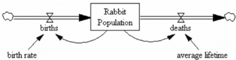
Following the successful completion of the initial exercises with the simple population model, participants are then encouraged to think of its possible modifications and enhancements. The original model on the Ventana website simulates the populations of rabbits (Figure 3), but similar principles apply to a wide range of other organisms. The learners are encouraged to adapt the population model in that respect, and a number of references are suggested where similar models have been used for algae, protozoa, cyanobacteria and diatoms [8, 13, 14, 22, 23] and zooplankton and fish [24]. Furthermore, it is emphasised that with certain modifications this modelling approach could be applied to human populations, and the learners are invited to introduce the processes of emigration and immigration, and to adapt the modified model to describe the processes relevant to the population of Ebbsfleet Garden City (Figure 4). This exercise (which would be attempted during the tutorial or otherwise suggested as homework) provides a link between Session 1 and Session 2, devoted to the exploration of the Ebbsfleet SDM using more advanced tools.
Figure 3. Diagram of a simple population model used to exemplify the basics of SD modelling and to build up the understanding of the stocks and flows concepts
Figure 4. Diagram of the modified population model adapted to represent time series of changes in residents numbers in Ebbsfleet Garden City. Note two additional flows (immigration and emigration) affecting the dynamics of the population compartment
Session 2: Exploration of the Ebbsfleet SDM: designing and running scenarios, and making modifications
This tutorial session is designed to facilitate the learners experience of running, adjusting and further developing more complex models, using the example of the Ebbsfleet Garden City model. This model contains four differential and a number of algebraic equations, and has previously been used both as a research tool, and for teaching the SD modelling techniques. The diagram and a brief description of the model are given in Table 2. The increased structural complexity of the model leads to the increased behavioural complexity, and session 2 is designed to facilitate the learners exploring this complexity using more advanced tools available in the Vensim interface.
The recommended time to complete this session is 3 hrs. It is suitable for either classroom or online delivery, or for self-study. The recommended preliminary reading for this session are Refs. [17] and [18], as they are extensively referred to during the tutorial. An important prerequisite for this session is completion of Session 1 (or previous experience with ‘stock & flow’ models and the Vensim-type software). Also, before the session, the participants are expected to read the paper describing in detail the original model [17] and the more recent paper which gives an example of how to introduce changes to the model structure [18].
Table 2. List of key variables included in the Ebbsfleet SD model. GWR = Greywater Reuse, RWH = Rainwater Harvesting, GW = Greywater, CSOs = Combined Sewer Overflows
|
Variable |
Description |
|
Cost of Greywater Reuse (GWR) |
Cost of GWR systems, depending on unit cost and on the existence of economic subsidies |
|
Cost of Rainwater Harvesting (RWH) |
Cost of RWH systems, depending on unit cost and on the existence of economic subsidies |
|
Combined Sewer Overflows (CSOs) |
Yearly volume of water in combined sewer systems overflow events |
|
Development rate |
It defines the yearly rate of the Urban Development, restricting the Urban Development transfer into the Population. It is set to 0.15 |
|
Environmental awareness |
It is mainly related to the rate of change set by ‘Inflow EA’. The maximum value of the ‘Environmental awareness’ stock is capped at 0.8 (‘EA cap’) and no further increase takes place beyond this value |
|
Greywater reuse (GWR) |
This variable describes the volume of Greywater (GW) reused on a yearly basis for residential purposes only |
|
Greywater (GW) in combined sewer system |
Defines the difference between the total GW produced and the volume that is reused |
|
GWR acceptability |
It defines the global level of acceptability and potential uptake of GWR systems, depending on cost and on the environmental awareness |
|
Outdoor residential use of potable water |
Volume of water that is needed on yearly basis for outdoor uses |
|
Population |
It defines the evolution of the population in the area, with an ‘increase rate’ related to the progress of ‘urban development’. An average of 3 persons per household is assumed (total number of 12,000 houses) |
|
Potable Water Balance |
All inflows and outflows are considered. Negative values identify a potential water supply deficit. Positive values instead represent the potential volume of water that can be saved in different scenarios |
|
Rainwater Harvesting (RWH) |
The volume of RWH, mainly depending on ‘RWH properties #’, an expected unit efficiency and rainfall conditions |
|
Regulatory policy instruments |
Global effectiveness of the selected policy instruments, calculated as their average value |
|
Socio-Environmental incentivising policy instruments |
Defines a time delay in the impacts of the ‘Educational programmes and events for sharing best practices’ |
|
(Water) Balance |
This component depends primarily on the difference between the ‘Potable water demand’ and the ‘Yearly water supply’. It is directly affected by the ‘Outdoor residential use of potable Water’, as well as by the ‘GWR’ and ‘RWH’ |
|
Water bills |
Water bills (stock) is computed from the identification of a baseline unit value (initial value 0.8073 £/l) and potential causes for its increase |
|
Water in combined sewer systems |
Total volume of water that flows (yearly) in the combined sewer system |
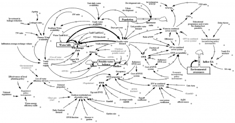
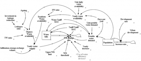
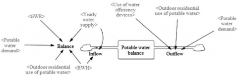
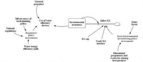
The diagram of the model version used for this course is shown in Figure 5 and the diagrams of the specific submodels are given in Appendix 1. The list of the most important variables (including stocks) is given in Table 1. A full list of variables, along with units, is provided in Appendix 2. In order to support a better understanding of the diagram, it has been structured using 4 sub-models, which focus on the key dynamics related to the following specific themes, namely: (i) potable water balance; (ii) water availability and demand; (iii) rainwater harvesting (RWH) and grey water reuse (GWR); (iv) environmental awareness. It should be noted that although the model is based on the original research version of the model published in the study on [17], the version presented in this paper includes modifications detailed in the study on [18] and has been further enhanced with explicit representation of all the constants and auxiliary variables, as well as their units. Such a detailed explicit representation was deemed necessary after the initial trials of this course following the feedback from the learners who found that the units of the original research version was, in places, somewhat difficult to follow.
The model computes a basic hydraulic water balance at urban level (i.e., a comparison between water demand and water supply) performed at a yearly time-scale, and considering an aggregated behaviour over the whole urban area (i.e., no individual or micro-behaviours are modelled). Following the inputs provided by the stakeholders, specific attention is given to the analysis of the role of sustainable water saving/management strategies such as RWH and GWR. Following the stock and flow diagramming notations, the model comprises stocks (i.e., accumulations related to real-world categories such as material or knowledge, drawn with rectangles), flows (rates of change in the value of stocks, drawn with an arrow with a valve), variables (dynamic variables, used to define intermediate concepts and changing instantaneously according to a formula and numeric constants) and links (arrows denoting a dependency between elements of a stock and flow diagram).
Figure 5. Diagram used in the teaching version of the Ebbsfleet model
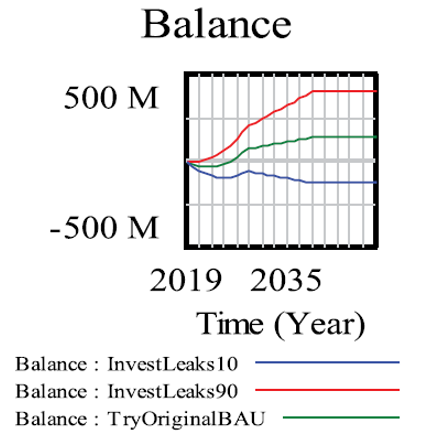
Figure 6. Exploring changes in water balance due to different levels of investment in leakage reduction. ‘TryOriginalBAU’ refers to the scenario ‘Business as Usual’, whilst ‘InvestLeaks90’ and ‘InvestLeaks10’ refer to the scenarios corresponding to, respectively, 90% and 10% of maximum possible investment in tackling the leakages
The learners start by running the model with the already entered default inputs. Then they are encouraged to make changes to some of the parameter values and observe how that would affect the dynamics of the modelled variables. For example, it is suggested to examine what would happen if the ‘investment in leakage reduction’ were changed from the default value. The results for the water balance are displayed in Figure 6. It is obvious that good investment in tackling leakages results in water savings and hence the healthier balance, whilst ignoring the problem would lead to water wastages and the deficit of this important resource.
In the next part of the tutorial the participants are suggested to introduce changes into the model’s structure and simulate a set of scenarios detailed in the study on [18] whilst trying such techniques as ‘SyntheSim’, ‘Causes strip’ and ‘Runs Compare’ tools, among others. This process helps the learners to acquire skills of searching for the causes of the observed patterns, and to understand why a given behaviour emerges from specific combinations of parameters.
The modified model links the pricing policy with the increase in ‘environmental awareness’ of the public. Although the model’s behaviour is complex, the expected patterns are intuitive and described in detail in the teaching materials supplied. Whilst completing these exercises the participants are ‘learning by doing’ and ‘learning by example’ (sensu [25]).
Initial trial runs of the SDM course presented here were offered to the members of the EPSRC Urban Flood Resilience (UFR) research consortium http://www.urbanfloodresilience.ac.uk/. The teaching materials were subsequently modified based on this experience, and the course was offered to a British Environmental Consultancy and to staff of the Ecology Department in Karazin University (Ukraine). Following that, an online feedback form was used to gauge the perception of the learners on the overall usefulness of the course and the specific sessions, and to collect ideas on potential improvements. The constructive positive feedback received from participants was encouraging, and helped to introduce further modifications aiming to facilitate knowledge transfer and enhance the learners’ experience. Specifically, the session on system thinking was introduced partly in response to the feedback provided by the participants. This valuable session was, however, made optional reflecting on the fact that the initial delivery of the course did not have such a session. It should be noted that more advanced participants were able to complete the main exercises without prior supplementary reading; however, all the participants (including those who studied the Systems Thinking materials after completing the other sessions) commented highly on its usefulness and merits.
It should be noted that the course described in this paper has, to date, been applied only in a limited number of trial, pilot studies. In all the applications the course was optional, and there was no formal assessment. Currently, there is an intention (subject to logistics) to offer the course in the Royal Botanic Garden Edinburgh (RBGE) for the master students studying plant sciences; discussions are also under way for potential delivery to the students of environmental and civil engineering at the Imperial College. Furthermore, having attended the course presented here, staff of Karazin University have been inspired to compile their own course in SD and ecological modelling; they are currently adapting the teaching materials presented here and aiming to develop them further for an in-person delivery of an enhanced course to their ecology students.
It should also be noted that this course is introductory; it provides the learners with basics and initial practical experience, but does not cover many of the more advanced topics. However, by applying the ‘learning-by-doing’ strategy, the course stimulates the learners to develop their skills further through self-learning and practical applications. During the initial trial sessions it has been observed that the participants were gradually developing their skills whilst transitioning from the rabbit population model to the considerably more complex Ebbsfleet water management model. Typically, the important qualitative change in the participants’ systems thinking and modelling skills becomes apparent after the exercise when they come back to the population model to adapt it for representing temporal changes in the number of Ebbsfleet residents. This qualitative change tends to become particularly obvious when the participants start trying to develop their own application.
Furthermore, the content of the course is generic. The specific model examples used in our course are relevant to ecology, engineering and social sciences. Consideration of the simple population model is relevant to many applications and disciplines; that will facilitate the knowledge transfer for learners with a wide range of backgrounds and help them to gain the initial basic modelling skills. Application of the Ebbsfleet SDM considers the complex interlinked problems of urban water management (UWM). These problems are pertinent not only for the Ebbsfleet case study, but are characteristic for UWM in general, and similar modelling case studies are currently being conducted elsewhere. The ability to understand this complexity is indispensable for finding successful solutions to interrelated environmental and social issues [17, 18, 26-28], and is key to the sustainable development of modern cities [17, 29-31]. System dynamics studies are very useful in that respect and have a potential added value of engaging practitioners and the public in further developments of the resulting models [17, 18, 32]. The research presented here has practical implications in helping to achieve and promote the multiple benefits of blue-green infrastructure including its intangible societal values, and is therefore contributing to the ongoing development of the Blue-Green Cities conceptual framework [28, 30, 33-35].
Simulation modelling is helpful for understanding the patterns of interactions between and within complex social and environmental systems [2, 4]. SD modelling is particularly useful in that respect as it provides a convenient tool for the analysis of interactions between system components and the assessment of a wide range of potential scenarios related e.g., to technological innovations, policy interventions, climate change and meteorological variability, as well as social and economic issues, among others [4, 17].
Adequate modelling skills are essential for modern science, and can also be of good use for a wide range of professional practitioners, politicians and general public. However, outside physics and math departments, modelling is often perceived as daunting and tedious activity. Nevertheless, the process of learning basic notions of Systems Thinking and SD modelling skills can be considerably facilitated through hands-on experience with modern interactive tools in a play-like activity. The concise course on SDM and Systems Thinking presented here provides a useful example in that respect.
Our teaching materials utilise the Vensim software which has proved convenient for building basic ‘stock and flow’ models. Importantly, this software is free for non-commercial use, which is an obvious advantage and has been a major factor determining the choice. However, there is no reason why interested users could not re-implement the models used in other interactive modelling software such as Stella, Madonna or Simile. It would also be fairly straightforward to compile both the population model and the Ebbsfleet SDM in most programming languages (e.g., Fortran, Visual Basic, C, Matlab) given that all the equations have been explicitly documented. In our opinion, Simulink and Matlab might be particularly convenient for that. By approximating ordinary differential equations by difference equations, the model could be sufficiently simplified for an easy implementation in a spreadsheet, such as e.g., ‘Calc’ (for Linux), ‘Numbers’ (for Mac) or ‘Microsoft Excel’ (for Windows). The latter software in addition to the spreadsheet capabilities also has a built-in version of BASIC (i.e., VBA), and may, therefore, be particularly useful for debugging the spreadsheet model and comparing its output with the version based on differential equations. Hence in addition to Vensim, further extended versions of the course should aim to use a number of other software packages, subject to logistical and financial constraints.
The course presented here has been designed for parsimonious delivery and is, therefore, based on a limited number of examples. Nevertheless, it should be noted that the teaching materials presented here are, of course, open to adjustments and further development. They could, therefore, be easily expanded to incorporate more case studies, more complex modelling functions and modelling techniques. Addition of case studies describing environmental dynamics in continental shelf seas [36, 37], water quality in rivers [38, 39], hydrology and ecology of lakes [7] and urban ponds [40, 41], and energy budget in waste management operations [5, 10, 42, 43] are all currently being considered. It should also be noted that although the concise course presented here has been based on only two SDMs, it has, however, been designed to give the learners important skills for approaching SD modelling and drafting their own basic models. Typically, short environmental modelling courses focus on ‘what if’ scenarios investigating changes in the input data and uncertainty of parameter values. Such activities are invaluable for the developing learners understanding, and have been incorporated fully in the teaching materials of the course presented here. In addition, however, our course contains a number of exercises aiming to introduce changes in the model’s structure, followed by subsequent observations of changes in the simulated patterns and discussion of further potential modifications. The examples of simple structural changes clearly demonstrate that both the processes represented in the models and their interlinkages can be easily adjusted, and the system boundaries can be easily broadened. Consequently, a combination of the course activities prepares the learners for developing their own models representing any processes of their choice. A logical extension of the course may, therefore, contain detailed information on other widely used modelling functions and tools, and also ‘student projects’ sessions, where participants would have an opportunity to create and present their own models, and to receive feedback from their classmates [44] and the tutors, which is an essential part of the education process [45].
Currently, all the teaching materials for the course presented here are compiled in a distribution bundle, available from https://www.researchgate.net/publication/365345624_EbbsfleetSDMtutorialBundleNov2022. As described above, the course is suitable for either online or in-class delivery, or for self-study. The training materials are centred on the development of key modelling skills, and incorporate an interdisciplinary modelling case study [17, 18]. To date, the participants of the trial runs came from a variety of backgrounds and levels of experience, including those completely new to mathematical modelling.
We expect that, with simple modifications, this concise course should be of use if integrated in undergraduate and master level modules related to a wide range of fundamental and applied disciplines, including e.g., Ecology, Geography, Engineering, Social and Environmental Sciences. As our experiences show, it will also be useful for training in ecological and environmental consultancies, as well as for a wider range of practitioners including private businesses, politicians and government officials. The teaching materials presented here may be particularly useful for horticultural and green infrastructure projects involving participatory approach [17, 28, 46]. Even more widely, the freely downloadable concise course giving the learners hands-on experience in Systems Thinking and the basic ‘do-it-yourself’ skills of ecological and environmental modelling, is likely to be of value for the interested members of general public. It is expected that University students and other SDM users will not only benefit from enhancing their understanding of the complexity of the specific problems considered by the examples used but will also gain basic system modelling skills through ‘learning by doing’; ultimately, the whole society benefits from the increased level of knowledge and analytical thinking skills of its members.
All the supplementary materials for this paper are freely available for download from https://www.researchgate.net/publication/365345624_EbbsfleetSDMtutorialBundleNov2022.
The research presented here was, in part, performed as a follow up of an interdisciplinary project undertaken by the Urban Flood Resilience Research Consortium (http://www.urbanfloodresilience.ac.uk/). The work was supported by the UK Engineering and Physical Sciences Research Council (grant numbers EP/ P004180/1, EP/P003982/1 and EP/P004318/1). Preparation of this manuscript has also benefitted from RBGE core funding. Comments of Colin Thorne and two anonymous reviewers helped to improve the manuscript. We are also grateful to all participants of the trial runs, and to Andrea Snelling, Simon Harrison and Andrey Achasov for their involvement in organising the training sessions.
Appendix 1. Diagrams of Submodels Constituting the SDM Presented in Figure 5
Submodel 1. Water demand and availability, water bills
Submodel 2. Potable water balance
Submodel 3. Environmental awareness and incentivising instruments
Submodel 4. RWH and GWR
Appendix 2. Description of variables used in the updated Ebbsfleet urban water management model. See text and supplementary materials for further information.
The model’s diagram is displayed in Figure 5 and the submodels in Appendix 1.
For clarity the following acronyms were used in the table below: GWR = Greywater reuse, RWH = Rainwater Harvesting, GW = Greywater, CSOs = Combined sewer overflow:
|
Variable |
Units |
Description |
|
Ageing |
Dimensionless [0-1] |
It describes the level of ageing of the infrastructural system. It ranges between 0 (new) and 1 (very old/out of service) |
|
Average yearly rainfall |
mm/Year |
Provides a value of the average Yearly rainfall over the area (Measured) |
|
Conversion coefficient |
l/(m2*mm) |
Converts the mm of rainfall per unit area (m2) to litres |
|
Cost of GWR |
£/(house*Year) |
Cost of GWR systems, depending on unit cost and on the existence of economic subsidies |
|
Cost of RWH |
£/(house*Year) |
Cost of RWH systems, depending on unit cost and on the existence of economic subsidies |
|
CSO ratio |
Dimensionless [0-1] |
Fraction of the water flowing into combined sewer system that ultimately contributes to CSOs |
|
CSOs |
litres/Year |
Yearly volume of water in combined sewer systems overflow events |
|
Days per year |
days/Year |
Defines the number of days (365) in the time step considered (year) |
|
Delay factor |
Year |
Defines a delay (currently 5 years) for the transfer of Educational programmes into Socio-Environmental incentivising policy instruments |
|
Development rate |
persons/(houses*Year) |
It defines the yearly rate of the Urban Development, restricting the Urban Development transfer into the Population. It is set to 0.15 |
|
EA cap |
Dimensionless [0-1] |
Upper limit of the Environmental Awareness |
|
Educational programmes and events for sharing best practices |
Dimensionless [0-1] |
Effectiveness/frequency of implementation of the selected policy instrument |
|
Effectiveness of local planning policy |
Dimensionless [0-1] |
Effectiveness/level of implementation of the selected policy instrument |
|
Efficiency |
Dimensionless [0-1] |
Efficiency factor of the sewer system (currently 0.85) |
|
Environmental awareness |
Dimensionless [0-1] |
It is mainly related to the rate of change set by ‘Inflow EA’. The maximum value of the ‘Environmental awareness’ stock is capped at 0.8 (‘EA cap’) and no further increase takes place beyond this value |
|
Expected unit RWH |
litres/(house*Year) |
Reference value of yearly water harvested per house, currently set to 1,000 |
|
Fraction of GWR |
Dimensionless [0-1] |
It defines a reference value for the houses equipped with GWR systems |
|
Garden size |
m2 |
Reference size of the garden (currently 50) |
|
Greywater reuse (GWR) |
litres/Year |
This variable describes the volume of Grey Water (GW) reused on a yearly basis for residential purposes only |
|
GW in combined sewer system |
litres/Year |
Defines the difference between the total GW produced and the volume that is reused |
|
GWR acceptability |
Dimensionless [0-1] |
It defines the global level of acceptability and potential uptake of GWR systems, depending on cost and on the environmental awareness |
|
Houses w. garden |
houses |
Fraction of new households with a garden |
|
Increase rate |
persons/Year |
It defines how the Urban Development produces an increase in population (it has an upper limit of 35000, i.e., approx. 3 persons/house) |
|
Infiltration-storage recharge volume |
litres/Year |
It depends on the potential future developments of the water supply system, and is activated for a scenario analysis only |
|
Inflow |
litres/Year |
Positive yearly contribution to the Potable Water Balance |
|
Inflow EA |
1/Year |
Yearly increase rate of the Environmental Awareness |
|
Investment in leakage reduction |
Dimensionless [0-1] |
It quantifies the investment performed to preserve system conditions. It ranges between 0 (no investment) and 1 (significant investment) |
|
Investment in WWTPs |
Dimensionless [0-1] |
Level of investment in WWTPs, from 0 (absent) to 1 (full) |
|
Leakages ratio |
Dimensionless [0-1] |
It computes an expected ratio of leakages depending on the age of the system and the investments performed. It ranges between 0 (no leakages) and 1 (system out of service) |
|
Metered properties |
Dimensionless [0-1] |
Ratio of the Metered properties out of the Total properties |
|
National regulations |
Dimensionless [0-1] |
Effectiveness/level of implementation of the selected policy instrument |
|
Occupancy |
persons |
Average occupancy of the properties (3) |
|
Outdoor residential use of potable water |
litres/Year |
Volume of water that is needed on yearly basis for outdoor uses |
|
Outflow |
litres/Year |
Negative yearly contribution to the Potable Water Balance |
|
Population |
persons |
It defines the evolution of the population in the area, with an ‘increase rate’ related to the progress of ‘urban development’. An average of 3 persons per household is assumed (total number of 12,000 houses) |
|
Potable Water Balance |
litres |
All inflows and outflows are considered. Negative values identify a potential water supply deficit. Positive values instead represent the potential volume of water that can be saved in different scenarios |
|
Rainfall |
mm/Year |
Provides a value of the Yearly rainfall over the area for the simulation |
|
Rainwater Harvesting (RWH) |
litres/Year |
The volume of RWH, mainly depending on ‘RWH properties #’, an expected unit efficiency and rainfall conditions |
|
Ratio of GW |
Dimensionless [0-1] |
Fraction of drinking water becoming GW (currently set to 0.7) |
|
Reference GWR cost |
£/(house*Year) |
Unit reference cost of GWR system, representing the upper limit over which it might become uneconomic. Currently the value is set to 15000 |
|
Reference RWH cost |
£/(house*Year) |
Unit reference cost of RWH system, representing the upper limit over which it might become uneconomic. Currently the value is set to 5,000 |
|
Regulatory policy instruments |
Dimensionless [0-1] |
Global effectiveness of the selected policy instruments, calculated as their average value |
|
Runoff coefficient |
Dimensionless [0-1] |
Average fraction of impervious area in the study area. Currently 0.5 |
|
RWH fraction |
Dimensionless [0-1] |
Defines a target/reference value of properties equipped with RWH systems. Currently set to 0.7 |
|
RWH properties # |
houses |
The number of households that are equipped with RWH systems |
|
RW in combined |
litres |
Volume of RW that flows into the combined sewer system |
|
Socio-Environmental incentivising policy instruments |
Dimensionless [0-1] |
Defines a time delay in the impacts of the ‘Educational programmes and events for sharing best practices’ |
|
Southern Water availability |
litres/Year |
Water volume that is needed on a yearly basis, provided by Southern Water |
|
SuDS effectiveness |
Dimensionless [0-1] |
Provides a global estimated effectiveness of the SuDS over the area, ranging from 0 (not effective) to 1 (fully effective) |
|
SW ratio |
Dimensionless [0-1] |
Ratio of the water volume that is needed on a yearly basis, provided by Southern water. Currently it is set to 1/3 |
|
Tariff/Tariff BAU |
Dimensionless |
It defines in a simplified form the structure of the tariff with respect to ‘Business as Usual’ (BAU) conditions |
|
Thames Water availability |
litres/Year |
Water volume that is needed on a yearly basis, provided by Thames Water |
|
TW ratio |
Dimensionless [0-1] |
Ratio of the water volume that is needed on a yearly basis, provided by Thames Water. Currently it is set to 2/3 |
|
Unit area |
m2/house |
Unit reference area drained for each property |
|
Unit daily water availability |
litres/(person*day) |
It defines the reference/expected daily water availability for domestic use. The BAU considers 120 litres/(person*day) |
|
Unit potable water demand |
litres/(person*day) |
It defines the reference/expected daily water demand for domestic use. The per capita value is set as 120 litres/(person*day) |
|
Upper WB limit |
£/litre |
It defines the upper limit of the Water Bill |
|
Urban Development |
# households |
Total number of households that are going to be built in the area throughout the development period. The value is set to 12000 |
|
Use of water efficiency devices |
Dimensionless [0-1] |
Identifies the use of water efficiency devices, combining metered properties, environmental awareness and regulatory policy instruments |
|
(Water) Balance |
litres/Year |
This component depends primarily on the difference between the ‘Potable water demand’ and the ‘Yearly water supply’. It is directly affected by the ‘Outdoor residential use of potable water’, as well as by the ‘GWR’ and ‘RWH’. |
|
Water bills |
£/litre |
Water bills (stock) is computed from the identification of a baseline unit value (initial value 0.8073 £/l) and potential causes for its increase |
|
Water-energy efficiency audit |
Dimensionless [0-1] |
Effectiveness/level of implementation of the selected policy instrument |
|
Water in combined sewer systems |
litres/Year |
Total volume of water that flows (yearly) in the combined sewer system |
|
Water Tariff BAU |
£/litre |
It defines the current value of the Water tariff |
|
WB change rate |
£/(litre*year) |
It defines the yearly change rate of the water tariff |
|
WD threshold |
Dimensionless [0-1] |
Defines the upper limit of potable Water Demand that does not activate an increase in water tariff |
|
WWTPs |
litres/Year |
Volume of water in WWTPs |
|
Yearly water availability |
litres/Year |
Calculates the volume of water that should be made available on yearly basis, given the unit daily water availability and the population |
|
Yearly Water supply |
litres/Year |
The water supply depends on the availability from ‘Thames Water’ and ‘Southern Water’, and on the ‘Infiltration-storage-recharge volume’ |
|
Yearly increase |
£/(litre*Year) |
Yearly increase level of the Water Bill |
[1] Sternman, J. (2000). Business Dynamics: Systems Thinking and Modeling for a Complex World. Irwin/McGraw-Hill.
[2] Forrester, J.W. (1961). Industrial Dynamics. MIT Press.
[3] Forrester, J.W. (1968). Principles of systems. Portland Productivity.
[4] Meadows, D.H, Meadows, D.L., Randers, J., Behrens, W.W. (1972). The Limits to Growth. Washington, DC: Potomac Associates.
[5] Krivtsov, V., Wäger, P.A., Dacombe, P., Gilgen, P.W., Heaven, S., Hilty, L.M., Banks, C.J. (2004). Analysis of energy footprints associated with recycling of glass and plastic—case studies for industrial ecology. Ecological Modelling, 174(1-2): 175-189. https://doi.org/10.1016/j.ecolmodel.2004.01.007
[6] Krivtsov, V., Watling, R., Walker, S.J.J., Knott, D., Palfreyman, J.W., Staines, H.J. (2003). Analysis of fungal fruiting patterns at the Dawyck Botanic Garden. Ecological Modelling, 170(2-3): 393-406. https://doi.org/10.1016/S0304-3800(03)00241-2
[7] Krivtsovi, V., Bellinger, E., Sigee, D. (2002). Water and nutrient budgeting of Rostherne Mere, Cheshire, UK. Hydrology Research, 33(5): 391-414. https://doi.org/10.2166/nh.2002.0015
[8] Krivtsov, V., Bellinger, E., Sigee, D. (2000). Incorporation of the intracellular elemental correlation pattern into simulation models of phytoplankton uptake and population dynamics. Journal of Applied Phycology, 12: 453-459. https://doi.org/10.1023/A:1008166914469
[9] Krivtsov, V., Dacombe, P., Kozenko, E.P., Zotova, E.A., Pak, L.N., Heaven, S., Banks, C.J. (2008). Current advances in waste management: Examples from Kazakhstan and the UK. In J.R. Lavelle (Ed.), Waste management: Research, technology and developments. NovaScience. ISBN 978-1-60021-256-9.
[10] Dacombe, P., Krivtsov, V., Banks, C., Heaven, S. (2004). Use of energy footprint analysis to determine the best options for management of glass from household waste. In Sustainable Waste Management and Recycling: Glass Waste, Thomas Telford Publishing, pp. 265-272.
[11] Dacombe, P., Krivtsov, V., Banks, C.J., Heaven, S. (2005). Energy and material flow of waste-processing operations. Proceedings of the Institution of Civil Engineers - Engineering Sustainability, 158(1): 17-23. https://doi.org/10.1680/ensu.2005.158.1.17
[12] Krivtsov, V., Corliss, J., Bellinger, E., Sigee, D. (2000). Indirect regulation rule for consecutive stages of ecological succession. Ecological Modelling, 133(1-2): 73-81. https://doi.org/10.1016/S0304-3800(00)00281-7
[13] Krivtsov, V., Bellinger, E., Sigee, D., Corliss, J. (2000). Interrelations between Si and P biogeochemical cycles - a new approach to the solution of the eutrophication problem. Hydrological Processes, 14(2): 283-295. https://doi.org/10.1002/(SICI)1099-1085(20000215)14:2<283AID-HYP926>3.0.CO;2-9
[14] Krivtsov, V. (2001). Study of cause-and-effect relationships in the formation of biocenoses: their use for the control of eutrophication. Russian Journal of Ecology, 32: 230-234. https://doi.org/10.1023/A:1011354303389
[15] Skaza, H., Crippen, K.J., Carroll, K.R. (2013). Teachers’ barriers to introducing system dynamics in K-12 STEM curriculum. System Dynamics Review, 29(3): 157-169. https://doi.org/10.1002/sdr.1500
[16] Fisher, D.M. (2018). Reflections on teaching system dynamics modeling to secondary school students for over 20 years. Systems, 6(2): 12. https://doi.org/10.3390/systems6020012
[17] Pluchinotta, I., Pagano, A., Vilcan, T., Ahilan, S., Kapetas, L., Maskrey, S., O’Donnell, E. (2021). A participatory system dynamics model to investigate sustainable urban water management in Ebbsfleet Garden City. Sustainable Cities and Society, 67: 102709. https://doi.org/10.1016/j.scs.2021.102709
[18] Krivtsov, V., Pagano, A., Ahilan, S., O’Donnell, E.M.I.L.Y., Pluchinotta, I. (2021). Further development of the Ebbsfleet water management system dynamics model: Adjusting representation of processes and system boundaries, incentivising stakeholder re-engagement, and exploring potential for university teaching. In WIT Transactions on Ecology and the Environment, 251: 11-22.
[19] Sterman, J.D. (2012). Sustaining sustainability: creating a systems science in a fragmented academy and polarized world. Sustainability Science: The Emerging Paradigm and the Urban Environment, 21-58. https://doi.org/10.1007/978-1-4614-3188-6_2
[20] Groesser, S.N., Schaffernicht, M. (2012). Mental models of dynamic systems: taking stock and looking ahead. System dynamics review, 28(1): 46-68. https://doi.org/10.1002/sdr.476
[21] Vennix, J. (1996). Group Model Building: Facilitating Team Learning Using System Dynamics. John Wiley & Sons Inc.
[22] Krivtsov, V., Sigee, D., Corliss, J., Bellinger, E. (1999). Examination of the phytoplankton of Rostherne Mere using a simulation mathematical model. Hydrobiologia, 414: 69-74. https://doi.org/10.1023/A:1003854929525
[23] Krivtsov, V., Bellinger, E., Sigee, D., Corliss, J. (1998). Application of SEM XRMA data to lake ecosystem modelling. Ecological Modelling, 113(1-3): 95-123. https://doi.org/10.1016/S0304-3800(98)00137-9
[24] Krivtsov, V., Goldspink, C., Sigee, D.C., Bellinger, E.G. (2001). Expansion of the model ‘Rostherne’for fish and zooplankton: role of top-down effects in modifying the prevailing pattern of ecosystem functioning. Ecological modelling, 138(1-3): 153-171. https://doi.org/10.1016/S0304-3800(00)00400-2
[25] Bandura, A. (1971). Social learning theory. New York: General Learning Press.
[26] Ahilan, S., Guan, M., Wright, N., Sleigh, A., Allen, D., Arthur, S., Krivtsov, V. (2019). Modelling the long-term suspended sedimentological effects on stormwater pond performance in an urban catchment. Journal of Hydrology, 571: 805-818. https://doi.org/10.1016/j.jhydrol.2019.02.002
[27] CIRIA. (2019). Blue-green infrastructure - perspectives on water quality benefits. London: CIRIA C780b.
[28] CIRIA. (2019). Blue-green infrastructure - perspectives on planning, evaluation and collaboration. London: CIRIA C780a.
[29] Pagano, A., Pluchinotta, I., Giordano, R., Fratino, U. (2018). Integrating “Hard” and “Soft” infrastructural resilience assessment for water distribution systems. Complexity, 2018: 1-16. https://doi.org/10.1155/2018/3074791
[30] Krivtsov, V., Ahilan, S., Arthur, S., Birkinshaw, S., Dawson, D., Everett, G., Thorne, C. (2021). Blue-Green Cities: Achieving Urban Flood Resilience, Water Security, and Biodiversity. In The Palgrave Encyclopedia of Urban and Regional Futures, Cham: Springer International Publishing, pp. 1-8.
[31] Puchol-Salort, P., O’Keeffe, J., van Reeuwijk, M., Mijic, A. (2021). An urban planning sustainability framework: Systems approach to blue green urban design. Sustainable Cities and Society, 66: 102677. https://doi.org/10.1016/j.scs.2020.102677
[32] Maskrey, S.A., Mount, N.J., Thorne, C.R. (2022). Doing flood risk modelling differently: Evaluating the potential for participatory techniques to broaden flood risk management decision-making. Journal of Flood Risk Management, 15(1): e12757. https://doi.org/10.1111/jfr3.12757
[33] O'Donnell, E., Thorne, C., Ahilan, S., Arthur, S., Birkinshaw, S., Butler, D., Wright, N. (2020). The blue-green path to urban flood resilience. Blue-Green Systems, 2(1): 28-45. https://doi.org/10.2166/bgs.2019.199
[34] Fenner, R., O’Donnell, E., Ahilan, S., Dawson, D., Kapetas, L., Krivtsov, V., Vercruysse, K. (2019). Achieving urban flood resilience in an uncertain future. Water, 11(5): 1082. https://doi.org/10.3390/w11051082
[35] D'Arcy, B., Kim, L.H., Maniquiz-Redillas, M. (2017). Wealth Creation without Pollution: Designing for Industry, Ecobusiness Parks and Industrial Estates. IWA Publishing. https://doi.org/10.2166/9781780408347
[36] Krivtsov, V., Howarth, M.J., Jones, S.E., Souza, A.J., Jago, C.F. (2008). Monitoring and modelling of the Irish Sea and Liverpool Bay: An overview and an SPM case study. Ecological Modelling, 212(1-2): 37-52. https://doi.org/10.1016/j.ecolmodel.2007.10.038
[37] Krivtsov, V., Howarth, M.J., Jones, S.E. (2009). Characterising observed patterns of suspended particulate matter and relationships with oceanographic and meteorological variables: Studies in Liverpool Bay. Environmental Modelling & Software, 24(6): 677-685. https://doi.org/10.1016/j.envsoft.2008.09.012
[38] Dobson, B., Mijic, A. (2020). Protecting rivers by integrating supply-wastewater infrastructure planning and coordinating operational decisions. Environmental Research Letters, 15(11): 114025. https://doi.org/10.1088/1748-9326/abb050
[39] Dobson, B., Jovanovic, T., Chen, Y., Paschalis, A., Butler, A., Mijic, A. (2021). Integrated modelling to support analysis of COVID-19 impacts on London's water system and in-river water quality. Frontiers in Water, 3: 641462. https://doi.org/10.3389/frwa.2021.641462
[40] Krivtsov, V., Birkinshaw, S., Arthur, S., Knott, D., Monfries, R., Wilson, K., Monteiro, Y. (2020). Flood resilience, amenity and biodiversity benefits of an historic urban pond. Philosophical Transactions of the Royal Society A, 378(2168): 20190389. https://doi.org/10.1098/rsta.2019.0389
[41] Krivtsov, V., Birkinshaw, S., Forbes, H., Olive, V., Chamberlain, D., Lomax, J., Christie, D. (2020). Hydrology, ecology and water chemistry of two suds ponds: detailed analysis of ecosystem services provided by blue-green infrastructure. In 7th International Conference on Flood and Urban Water Management, FRIAR 2020, WITPress, pp. 167-178. https://doi.org/10.2495/FRIAR200151
[42] Krivtsov, V., Dacombe, P., Kozenko, E.P., Zotova, E.A., Pak, L.N., Heaven, S., Banks, C.J. (2008). Contemporary Applications of Interdisciplinary Waste Management Research: Case Studies of Algal Biodiversity in WSP and Energy Footprint of Municipal Wastes. International Journal of Energy, Environment, and Economics, 15(3-4): 183-204.
[43] Dacombe, P., Krivtsov, V., Banks, C.J., Heaven, S. (2005). Energy and material flow of waste-processing operations. In Proceedings of the Institution of Civil Engineers-Engineering Sustainability, 158(1): 17-23.
[44] Crouch, C.H., Mazur, E. (2001). Peer instruction: Ten years of experience and results. American Journal of Physics, 69(9): 970-977. https://doi.org/10.1119/1.1374249
[45] Hounsell, D. (2008). The trouble with feedback: New challenges, emerging strategies. Interchange, 2: 1-10.
[46] Krivtsov, V., D’Arcy, B.J., Sevilla, A.E., Arthur, S., Semple, C. (2021). Mitigating polluted runoff from industrial estates by SuDS retrofits: case studies of problems and solutions co-designed with a participatory approach. Sustainability, 13(22): 12357. https://doi.org/10.3390/su132212357