Hydrologic Modeling of Submarine Groundwater Discharge and Its Ecological Implications in a Coastal Lagoon under Data-Scarce Conditions

Groundwater stands as one of the most significant components of the water cycle, which is crucial for supporting all kinds of life and comprises one-third of the Earth’s freshwater supply. Population growth, coupled with climate change over the last century, has resulted in increased demand for groundwater [1] and in global declines in groundwater storage [2]. Several investigations have shown that overuse of this important resource without sustainable management and planning can result in a serious decline in groundwater levels [3, 4] as well as groundwater contamination [5, 6]. Thus, informed management of groundwater resources has become crucial for facing these increasing challenges. To effectively protect this precious resource, it is necessary to understand groundwater flow regimes and pollutant transport processes. Representing groundwater flow regimes and transport processes beneath the Earth’s surface is challenging due to uncertainty in aquifer hydraulic parameters and surface heterogeneity. As such, numerical modeling is an indispensable tool widely used to aid decision-making and sustainable management programs of groundwater sources. Recent advances in hydrologic modeling and computational capabilities have enabled the simulation of a wide range of complex groundwater flow and transport systems. However, without proper calibration, hydrologic models can easily produce nonunique, unstable, or insensitive simulations [7].

Calibration of groundwater hydrologic models is accomplished by iteratively adjusting the most sensitive parameters with the ultimate goal being to match simulated and observed data. After properly calibrating the model, its goodness and precision are usually evaluated by using additional field data to determine whether the model is able to mimic field conditions under boundary conditions different from the ones used initially to develop the model. Calibration involves the adjustment of uncertain and sensitive parameters, such as vertical hydraulic conductivity, K_v, that command extensive numerical calculations and calibration iterations. The most common strategy of model calibration involves the comparison of the simulated head results with the observed/measured head data known as calibration targets [8-10]. It is challenging to produce unique solutions based on a restricted number of well sites utilizing head values alone [11-13]. The more head data used for model calibration, the higher the calibration resolution. However, in many practical groundwater modeling problems, especially with regional models or in harsh environments such as saline environments, observed head data is usually scarce and very limited for many reasons. Insufficient field measurements (observed data) usually result in significant differences between simulated and observed data, since this causes a lack of appropriate representation of spatial variation in the hydraulic parameters of the modeled system. Subsequently, inadequate observational data pose significant constraints to the calibration of hydrological models, which subsequently compromises predictive accuracy and may ultimately impair the effectiveness of decision-making frameworks. It follows that a reliable strategy is needed to systematically achieve efficient hydrologic model calibration in regions with scarce observations.

Previous research has dealt with data scarcity conditions in groundwater modeling using several techniques and methodologies depending on site-specific conditions and the type of available data. Among these methodologies, lumped parameter groundwater modeling approaches have been adopted as alternatives to traditional physics-based models [14, 15]. Additionally, the integration of remote sensing products and literature data with conventional groundwater models has emerged as an established approach for improving simulation fidelity [16]. Some studies have used nested models and multi-index calibration [17], boundary condition analysis [18], or Earth observation [19]. Some other researchers have addressed the issues of data scarcity by using GRACE to strengthen model development [20, 21]. Another group of researchers has handled this problem through simplified methodologies, including employment of pilot points [22], Grey Models [23], parsimonious parameterization [24], head-guided zonation [25], stochastic reconstruction framework [26], and expert-based frameworks [27], all aimed at extracting additional data from scarce available data. To the best of the authors’ knowledge, studies that have employed interpolation techniques for increasing the reliability of groundwater modeling in data-sparse regions are very limited. A single study [28] was found in the literature in which groundwater depth is estimated in a data-limited area using optimal interpolation. Data collection in harsh environments, such as coastal lagoons, is usually challenging. It occasionally requires diving into the saline water for equipment installation in the sediments and the subsequent data collection. These difficulties pose significant limitations on the data collected for groundwater modeling efforts. Interpolation of limited data in such harsh conditions acts as a valuable tool for generating additional datasets for model calibration and validation. It can also introduce a significant reduction in time, effort, and cost that emanate from difficult data collection trips. However, the literature is lacking methodologies that utilize interpolation to extract head data in harsh environments, such as coastal aquifers with a saline environment, for calibrating flow regimes.

It is generally recognized that submarine groundwater discharge (SGD) has a strong potential to reshape these vital coastal ecosystems by impacting nutrient cycling and biodiversity [29]. In many coastal systems, SGD has been recognized as a major contributor to land-based nutrient fluxes, namely phosphorus and nitrogen, that exceed surface water fluxes by orders of magnitude [30]. For example, SGD was estimated to deliver more than 79% of dissolved inorganic phosphorus, nitrogen, and silica loads into Liaodong Bay, China [31]. SGD-driven nutrient fluxes can result in a significant imbalance of the nitrogen-to-phosphorus ratio (N/P). In many coastal systems, SGD has resulted in N/P ratios exceeding the Redfield ratio of 16:1, turning those ecosystems into phosphorus-limited environments and consequently driving eutrophication, growth of harmful algal blooms (HABs) [32], and fish kills [33]. Despite these negative impacts, SGD is reported to have several positive effects on coastal ecosystems, such as increased biodiversity in nitrogen-limited systems, fisheries, pollution attenuation, and coral calcification [32]. Thus, reliable estimation of SGD is critical for sustainable management of coastal environments.

This study focuses on developing a groundwater numerical model to simulate SGD into an unconfined coastal aquifer below a coastal lagoon known as the Banana River Lagoon (BRL). The environment at the site is predominantly saline, making it challenging to install and collect sufficient piezometric head and salinity data for model development. The lagoon width at the selected site is also relatively large, and thus, a higher resolution of data collection is needed to effectively represent the flow conditions. The study investigates the use of inverse distance weighting (IDW) interpolation of the limited data obtained from this data-scarce area by extracting additional synthetic data points from the interpolated surface. This methodology provides more data that serve the modeling process in two ways: 1) by providing more head targets for model calibration, and 2) by allowing model calibration to be evaluated statistically with more data rather than a limited number of data points.

3.1 Characterization and data collection procedure

The fieldwork initially involved installing a number of onshore and offshore clustered monitoring wells/piezometers and a benchmark (Figure 1) and delineating the lagoon bed profile along the selected transect (Figure 2). Groundwater levels measured at the onshore monitoring wells were used to define the groundwater divides and establish the transect’s horizontal extent up to the Atlantic Ocean. The transect spans a total horizontal distance of 6270 m, including 200 m through the groundwater divide on Merritt Island, 5730 through the lagoon water body, and 340 m of the Barrier Island to terminate at the Atlantic Ocean’s coast. The measured lagoon bed profile shows that the lagoon bottom at the study site ranges from 1 m to 3 m below the water surface (Figure 2). Groundwater levels collected from onshore piezometers on the Merritt and Barrier Islands were used to define the model boundary conditions. Eight stations of clustered piezometers were used to collect hydraulic head and lagoon water salinity below the transect, as depicted in Figure 2 (also shown as blue dots in Figure 1(c)). Each station contained a cluster of two monitoring piezometers at different depths ranging from 1.17 m to 3.66 m. An additional piezometer, deeper than the others (6.70 m), was later installed at the western station, bringing the total number of piezometers to 17. Table 1 provides more details on the horizontal locations measured from the Westshore stations (WS) and the screen elevation of each piezometer in NGVD29. Eight additional samples were collected from the lagoon surface water at sites corresponding to the eight monitoring stations at the lagoon bed elevations (Table 1). Adding those lagoon bed samples to the ones collected from the piezometers, a total of 25 samples were obtained during each sampling campaign. Temporal groundwater salinity ranges measured at the 25 locations, the average temporal lagoon water salinity, and the measured temporal lagoon water elevation are presented in Table 2. Owing to the difficulty of fieldwork in such a saline environment, the installation of deeper piezometers wasn’t feasible. Moreover, given the relatively large width of the lagoon, the number of monitoring points is relatively scarce to achieve reliable model calibration and validation. All salinity measurements were accomplished using a YSI 85 probe with a range of 0–180 ppt. Hydraulic head and salinity data were observed during three sampling dates conducted in July 2014, October 2014, and May 2015. The conversion of observed groundwater hydraulic heads below the lagoon to equivalent freshwater heads was necessary to account for salinity effects after generating the interpolated equipotential contour maps. This conversion was accomplished using Eq. (1).

${{H}_{fresh}}=\frac{{{\rho }_{salt}}}{{{\rho }_{fresh}}}{{h}_{salt}}-\frac{{{\rho }_{salt}}-{{\rho }_{fresh}}}{{{\rho }_{fresh}}}H$          (1)

where, H_fresh represents freshwater head in m; h_salt represents seawater head in m; H stands for elevation in m; ρ_fresh = density of freshwater, taken as 1000 kg/m³; ρ_salt = density of seawater, taken as 1025 kg/m³.

tu_pian_4.png

Figure 2. Data collection piezometer cluster distribution underneath the lagoon bed

Sediment samples of the lagoon bed were collected from five of the monitoring stations to estimate the horizontal hydraulic conductivity (K_h) of the aquifer by the equation K_h = C(d₁₀)², where d₁₀ is the effective diameter, and C is an empirical constant. A horizontal hydraulic conductivity of 20 m/d was calculated by averaging the estimated conductivity at all sampling points.

Table 1. Sampling locations and screen depths of the offshore piezometers and bed points

Table 2. Groundwater salinity ranges, lagoon surface water elevation, and average lagoon water salinity

3.2 Model development and simulations

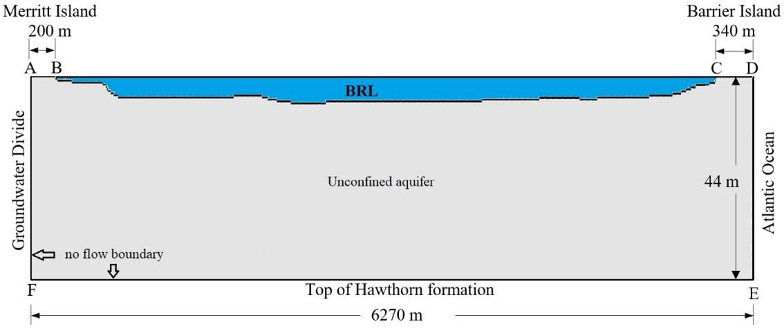
Numerical simulations were accomplished in the numerical environment of the groundwater flow and solute transport code SEAWAT [39]. The 2D cross-sectional domain of the model was 6270 m long and 44 m deep (Figure 3). The horizontal 6270 m stretch of the model covers the region from the Merritt Island groundwater divide to the Ocean. Boundaries A-B and C-D represent the fresh groundwater boundaries on Merritt Island and Barrier Island, respectively, and were represented in the model as constant head and concentration boundaries. The Hawthorn formation and the groundwater divide boundaries E-F and A-F, respectively, were assigned No-flow characteristics. The saltwater boundaries of the lagoon bed, B-C, and the Atlantic Ocean, D-E, were simulated by constant heads and concentrations. The normalized concentration of the sea boundary was 1, while the lagoon transect boundary was assigned a concentration of Cm/35000, with Cm representing the observed lagoon concentration based on seawater salinity of 35000. The initial concentration, Co, of the entire aquifer was set to zero, whereas the initial head was set to 44 m (total depth of the aquifer). The finite difference domain discretization included a single one-meter row, 176 columns, and 50 layers. Column spacing ranged from 4 to 40 m, and layer spacing ranged from 0.25 to 2.5 m. The model run was set to steady state with an implicit finite difference framework in the GCG solver. In total, three identically discretized steady-state models were developed, one for each sampling period (July 2014, October 2014, and May 2015). The only difference among the three models is that each uses boundary conditions representing a different stress period corresponding to a specific temporal sampling trip. An alternative approach would be to develop a single transient model incorporating all three stress periods. However, this would yield identical results to those obtained by the current approach, but the model would be more run-time demanding. Furthermore, in our current approach, viewing and post-processing results for a specific period is slightly more straightforward.

tu_pian_5.jpg

Figure 3. Model domain of the Banana River Lagoon (BRL) site developed in SEAWAT

3.3 Interpolation and uncertainty analysis of inverse distance weighting

The 25 piezometric head observations gathered in July 2014 were used to develop equipotential contours using IDW interpolation. Since the collected head data are limited relative to the model domain, 18 additional synthetic head values were extracted from the IDW surface for July 2014 and used with the original 25 points as head targets in model calibration to compensate for data scarcity. With a larger number of data points (larger sample), the reliability of the statistical analysis of model calibration can also be improved. The IDW interpolation-based synthetic points do not represent independent measurements. Instead, these points constitute mathematical approximations based on the actual field observations. As a result, using these synthetic points as spatial calibration constraints for the SEAWAT model may introduce spatial patterns and uncertainty to the model results.

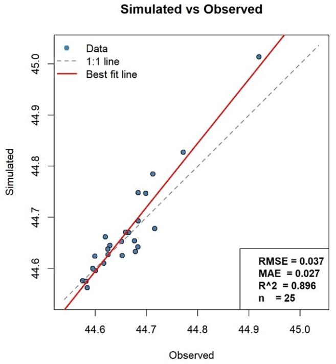
To evaluate the uncertainty inherent in the interpolation procedure, a leave-one-out cross-validation (LOOCV) procedure was employed. The LOOCV procedure was conducted by running the IDW interpolation of the actual field observations 25 times. In each run, one of the field observations was omitted, and its value was simulated by interpolating the rest of the field observations. The simulated observations were plotted against their actual field values, and the prediction error was quantified by RMSE, MAE, and R². The graphical and statistical procedures were performed using the R programming language.

The effect of uncertainty in interpolation-based points on the model SGD predictions was quantified using two calibration scenarios. One scenario used only the originally observed data as calibration constraints, while the second used the originally observed data plus the interpolated data as constraints. The difference between the two estimated SGD values was quantified and evaluated.

Due to their inherent uncertainty, the IDW-generated points were used as auxiliary calibration targets instead of independent targets. This was accomplished by downweighting these points in the objective function in the Parameter Estimation Software (PEST) calibration runs.

3.4 Calibration and validation

The procedure adopted in the calibration of the SEAWAT model was to use the July 2014 dataset for calibration and then validate the model using the October 2014 and May 2015 data. Since aquifer hydraulic conductivity usually controls groundwater flow [40], a sensitivity analysis was conducted to look into how sensitive the SEAWAT model was to K_h and K_v. During the sensitivity analysis, K_h was maintained at 20 m/d while using a single K_v for the entire domain. The K_v values tested during the sensitivity analysis were 0.2, 0.02, and 0.002 m/d. The sensitivity analysis aimed to calibrate the model and identify the K_v distribution that yields a close visual match between the simulated and observed groundwater head contours from July 2014. The model was initially calibrated using the PEST [41], and the calibration was further refined manually. PEST requires head calibration targets to optimize the objective function. The higher the number of targets, the higher the number of spatial constraints and the better the spatial conditioning of model calibration. Therefore, the model calibration was assessed in two scenarios: Scenario 1 with only the original 25 head observations as calibration targets, and Scenario 2 with the original 25 head observations plus the 18 IDW-based synthetic data points as targets. However, to compensate for the uncertainty inherent in the synthetic targets, they were downweighted in the PEST optimization of the objective function. The downweighting was based on the interpolation uncertainty analysis.

Following model calibration using a graphical comparison of the simulated and observed groundwater contours, the model goodness of fit was assessed statistically using the RMSE, t-test, and Nash-Sutcliffe efficiency (NSE) index [42]. There is no established standard for determining whether a model performs well or poorly, even though RMSE is frequently used in model calibration analyses with the aim of minimizing this measure. This is because the statistic's value usually varies depending on the units of measurement. At a 95 percent confidence level, the null hypothesis that the means of the simulated and observed groundwater heads are statistically equal was tested using a paired t-test. The goodness of fit between model results and measured heads is indicated by the NSE, which ranges from negative infinity to 1. While a value of zero or negative indicates that the mean of the measured data is a better predictor than the predicted values, a value of one indicates an ideal fit. An NSE value >0.5 would indicate a satisfactory match between the tested datasets.