Jackson Edgardo Perez Carpio* | Hugo Fernandez | Orlando Poma | Milda Amparo Cruz Huaranga | Jenny Sara Gavilán Santos | Juan Jesús Soria-Quijaite
© 2026 The authors. This article is published by IIETA and is licensed under the CC BY 4.0 license (http://creativecommons.org/licenses/by/4.0/).
OPEN ACCESS
Heavy metal contamination of river systems poses persistent risks to aquatic ecosystems and human health, particularly in watersheds affected by intensive mining and other anthropogenic activities. In this study, the spatial patterns and potential sources of heavy metal contamination in the middle Rímac River sub-basin, Peru, were investigated using an integrated framework combining chemometric analysis with explainable machine learning. Concentrations of 13 elements (Mg, B, Al, Cr, Mn, Fe, Cu, Zn, As, Cd, Sb, Ba, and Pb) measured at 21 monitoring stations were analyzed using principal component analysis, hierarchical cluster analysis, multidimensional scaling, and one-way analysis of variance, while random forest and extreme gradient boosting (XGBoost) classifiers were used to identify the elements contributing most strongly to spatial differentiation. Distinct spatial groupings and pronounced heterogeneity among monitoring sectors were consistently identified by the multivariate analyses. Analysis of variance showed significant differences among monitoring tracks for 12 of the 13 evaluated elements (p < 0.05), whereas Cr remained constant across all monitoring stations and was not subjected to analysis of variance (ANOVA). Random forest achieved an accuracy of 81%, while XGBoost achieved 76%. Variable-importance analyses highlighted complementary sets of elements associated with spatial discrimination, supporting the combined use of chemometric and explainable machine-learning approaches for environmental assessment and monitoring in mining-influenced Andean watersheds.
heavy metals, chemometrics, explainable machine learning, spatial patterns, river contamination, Rímac River basin, water quality assessment
Metal pollution in rivers is a global social problem that directly harms people’s health and the aquatic ecosystem [1]. This problem is closely linked to various human activities, including industry, agriculture, and mining. In this context, water quality monitoring has become a priority in order to ensure environmental and public health safety [2]. High concentrations of metals pose a threat to the aquatic ecosystem, affecting aquatic organisms and biota [3, 4]. Several studies show that rivers used for urban water supply are affected by agricultural run-off, industrial discharges, and mining; it is therefore necessary to carry out regular monitoring to assess water quality [5]. One of the major challenges facing the aquatic ecosystem is metal pollution resulting from human activities, which can exacerbate water stress and reduce the availability of fresh water for human consumption and agriculture [6, 7]. The Rímac River catchment supplies drinking water to more than ten million people in Lima, Peru; however, its capacity for hydrological regulation has been increasingly reduced due to pollution and soil degradation. This river basin faces various environmental challenges due to the exploitation of its resources and widespread pollution; as Lima’s main source of water supply, it provides approximately 80% of the water consumed by the city, but it is affected by the discharge of domestic, hospital, industrial, and mining effluents, which compromises the quality of the resource and the sustainability of the water system [8, 9].
The river basin is a key resource for sustainable development in the social, economic, and environmental spheres. The Andes are one of the main sources of these resources; however, river basins are increasingly being affected by human activities, which have a negative impact on water quality. It is therefore vital to carry out regular assessments to prevent risks, with the aim of protecting the ecosystem and the health of the communities that depend on these resources [10, 11]. Assessing the water quality of rivers is essential for the well-being of local communities, as these systems are used for a wide range of human activities. However, rising levels of pollution have caused water quality to deteriorate in various ways, making this a major environmental issue [12]. The Rímac River basin has a long history of water pollution, particularly in the upper sub-basin, where mining activities have been taking place since around 1930. Mining has contributed to the deterioration of water quality and has affected towns such as San Mateo, Chicla, Casapalca, and Matucana, located in the upper and middle reaches of the basin [13].
In this context, the hypothesis is put forward that heavy metal concentrations in the middle sub-basin of the Rímac River exhibit distinct spatial patterns associated with anthropogenic sources of pollution, and that chemometric techniques, complemented by explainable machine learning models, enable these patterns and their main sources of pollution to be effectively identified and interpreted. The aim of this research is to assess the spatial patterns and sources of heavy metal pollution in the middle sub-basin of the Rímac River, situated between the districts of San Mateo and Matucana, through the analysis of surface water samples and the application of chemometric tools and explainable machine learning models. The results can provide scientific information that contributes to the sustainable management of water resources, the protection of aquatic ecosystems, and the design of environmental monitoring and control strategies.
2.1 Study area
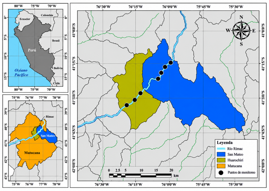
Lima, the capital of Peru, is considered the second-largest city in the world, situated in a desert region. The Rímac River is the main source of water for the population and for various activities. It rises in the snow-capped Paca peak of the Andes, at an altitude of approximately 5,508 meters above sea level, and flows for around 160 kilometers through its upper, middle, and lower basins, emptying into the Pacific Ocean in the Callao area [14]. The study area covers a stretch of approximately 30 km between the districts of San Mateo and Matucana, situated at the transition between the Upper Rímac sub-basin and the middle Rímac River basin. San Mateo is situated at the lower boundary of the upper sub-basin, while Matucana forms part of the middle section of the basin, making this a strategic stretch for monitoring water quality. Figure 1 shows the location of monitoring points along the Rímac River in San Mateo and Matucana.
Figure 1. Map of the location of monitoring points in the Rímac River basin in San Mateo and Matucana
2.2 Sample collection and analysis
A total of 21 surface water samples were collected from the middle sub-basin of the Rímac River, covering the districts of San Mateo and Matucana. The sampling points were selected on the basis of their potential exposure to anthropogenic activities, primarily mining and domestic discharges, with the aim of representing the spatial distribution of water quality. The geographical location of each sampling point was recorded using a global positioning system. Monitoring was carried out in February in accordance with the procedures set out in the National Protocol for the Monitoring of Surface Water Quality. Samples were collected in high-density polyethylene bottles, preserved by adding 2% nitric acid (HNO₃), and stored at 4 ℃ to preserve the samples until their analysis in the laboratory [15]. The assessment procedure comprises three stages: pre-monitoring, monitoring, and post-monitoring. The pre-monitoring phase involved planning the activities, selecting and coding the sampling points, defining the monitoring frequency and the parameters to be assessed, and preparing materials, equipment, and safety measures for the fieldwork. During the monitoring phase, a survey of the study area was carried out, sampling points were georeferenced, parameters were measured in situ, samples were collected and preserved, and the chain of custody was recorded; samples were then transported to the laboratory, thereby ensuring the quality of the data obtained. Finally, during the post-monitoring stage, the samples were analyzed at an accredited laboratory, the results were processed and validated, and the corresponding technical report was drawn up [16]. Table 1 shows the locations and coordinates of the monitoring stations.
Table 1. Locations and coordinates of the monitoring stations
|
Location |
Monitoring Points |
Coordinates |
|
|
N |
S |
||
|
San Mateo |
P1 |
8701536 |
359760 |
|
P2 |
|||
|
P3 |
|||
|
P4 |
8700129 |
358802 |
|
|
P5 |
|||
|
P6 |
|||
|
P7 |
8699800 |
358471 |
|
|
P8 |
|||
|
P9 |
|||
|
P10 |
8697516 |
357595 |
|
|
P11 |
|||
|
P12 |
|||
|
Matucana |
P13 |
8694728 |
353953 |
|
P14 |
|||
|
P15 |
|||
|
P16 |
8691385 |
350285 |
|
|
P17 |
|||
|
P18 |
|||
|
P19 |
8685818 |
342616 |
|
|
P20 |
|||
|
P21 |
|||
2.3 Contamination factor
The contamination factor is an index that assesses the degree of contamination for each metal individually, based on the ratio of the concentration measured in the sample to its background concentration or natural reference value.
$C F_i=\frac{C_i}{B_i}$ (1)
where, Ci is the measured concentration of the metal in the water, and Bi is the background concentration (or natural reference value) of the same metal.
The contamination factor was classified as follows:
Contamination factor < 1: Low pollution levels (within natural ranges).
1 ≤ contamination factor < 3: Moderate pollution factor.
3 ≤ contamination factor < 6: A significant source of pollution.
Contamination factor ≥ 6: Very high pollution level.
2.3.1 Background concentrations
Geochemical background values were used as reference concentrations to assess metal enrichment in surface waters. These values provide a baseline against which concentrations measured in the middle sub-basin of the Rímac River were compared. The selection of reference concentrations was based on published geochemical data regarding the natural occurrence of major and trace elements in river waters, taking into account global compilations of elemental concentrations in river waters. Because natural elemental concentrations can vary depending on lithology, weathering processes, hydrological conditions, and regional geology, these values were considered reference background concentrations rather than site-specific baseline concentrations for the Rímac River. The use of these reference values was supported by recent methodologies for determining natural background concentrations in surface waters. Table 2 shows the background concentrations of elements in river water used as reference values for contamination assessment.
Table 2. Background concentrations of elements in river water used as reference values for contamination assessment
|
Element |
Reference Concentration (mg/L) |
Reference Concentration (µg/L) |
|
B |
0.010 |
10 |
|
Mg |
4.100 |
4100 |
|
Al |
0.400 |
400 |
|
Cr |
0.001 |
1 |
|
Mn |
0.005 |
5 |
|
Fe |
0.670 |
670 |
|
Cu |
0.005 |
5 |
|
Zn |
0.010 |
10 |
|
As |
0.001 |
1 |
|
Cd |
0.001 |
0.1 |
|
Sb |
0.001 |
1 |
|
Ba |
0.010 |
10 |
|
Pb |
0.003 |
3 |
Source: Background concentrations compiled from global geochemical data on dissolved elements in river waters.
The elements were analyzed using inductively coupled plasma mass spectrometry. The laboratory responsible for the analysis has testing methods accredited by the National Institute of Quality in accordance with standard NTP-ISO/IEC 17025:2017, as well as by the International Accreditation Service ISO/IEC 17025:2017. Similarly, other studies have employed the same inductively coupled plasma mass spectrometry methodology for the analysis of metals [17].
2.4 Metal index
The metal index is a comprehensive index that assesses the overall water quality based on the presence of multiple metals. It takes into account the concentration of each element and its respective maximum permissible concentration.
$M_i=\sum_{i=1}^n C_i / M A C_i$ (2)
where, Ci is the concentration of the i-th metal in the sample analyzed, and MA is the maximum permissible concentration of the metal as specified in a standard or guideline (mg/L).
The metal index was interpreted as follows:
Metal index < 1: The water is considered to be pure or of excellent quality, and safe to use.
Metal index = 1: The water level is at the upper limit of what is permissible.
Metal index > 1: The water is polluted. The higher the index value, the greater the toxicity and the risk of adverse effects (particularly for human consumption or fishing).
2.5 Data analysis and statistical techniques
2.5.1 Statistical analysis
The data were analyzed using descriptive statistical techniques in order to understand the behavior of heavy metal concentrations in the middle sub-basin of the Rímac River [18]. Measures of central tendency and dispersion were calculated, including the mean, median, standard deviation, coefficient of variation, and minimum and maximum values. Subsequently, the distribution of the data and the relationship between the variables were assessed using correlation analysis and appropriate statistical tests. All analyses were carried out using the R software (version 4.4.0), with a significance level of p < 0.05.
Advanced statistical and chemometric methods have been widely used in metal pollution studies to identify relationships among variables and potential pollution sources [19, 20].
2.5.2 Chemometric analysis
Multivariate analysis techniques were applied with the aim of identifying spatial patterns, associations between variables, and possible sources of pollution. Principal component analysis was used to reduce the dimensionality of the dataset and identify the main factors responsible for the variability in heavy metal concentrations. Hierarchical cluster analysis enabled the monitoring stations to be grouped according to the similarity of their chemical characteristics, while multidimensional scaling facilitated the spatial representation of the relationships between the sampling points. The combined interpretation of these techniques made it possible to identify potential sources of pollution and assess the spatial distribution of heavy metals in the study area.
2.5.3 Explainable machine learning analysis
With the aim of improving the identification of pollution sources and enhancing the interpretation of results obtained through chemometric analyses, supervised machine learning models were implemented using the random forest and extreme gradient boosting (XGBoost) algorithms. These models were trained to identify spatial patterns of pollution and to determine the relative importance of environmental variables and heavy metal concentrations in the classification of monitoring stations.
3.1 Element concentrations in surface water in the Rímac River at San Mateo and Matucana
The Mg concentration ranged from 6.30 to 10.37 mg/L. An upward trend was observed from the sections located in San Mateo towards Matucana, indicating spatial variation across the catchment. This behavior may be associated with the presence of polymetallic and limestone deposits and with mining-related activities in the study area, where water-rock interactions and anthropogenic inputs may influence river chemistry.
Table 3. Concentrations (mg/L) of selected elements in surface water at the San Mateo and Matucana monitoring stations in the Rímac River basin
|
Town |
Track |
Code |
Monitoring Points |
Mg |
B |
Al |
Cr |
Mn |
Fe |
Cu |
Zn |
As |
Cd |
Sb |
Ba |
Pb |
|
San Mateo |
Track 1 |
E1 |
Upstream |
6.78 |
0.0274 |
0.08 |
0.0006 |
0.23138 |
0.1361 |
0.0117 |
0.0615 |
0.00423 |
0.00017 |
0.0031 |
0.05162 |
0.0084 |
|
E2 |
Central station |
6.30 |
0.0249 |
0.08 |
0.0006 |
0.21620 |
0.1246 |
0.0093 |
0.0518 |
0.00394 |
0.00015 |
0.0029 |
0.04723 |
0.0084 |
||
|
E3 |
Downstream |
6.80 |
0.0240 |
0.08 |
0.0006 |
0.23605 |
0.1445 |
0.0108 |
0.0601 |
0.00449 |
0.00018 |
0.0030 |
0.04997 |
0.0113 |
||
|
Track 2 |
E4 |
Upstream |
8.95 |
0.3702 |
0.07 |
0.0006 |
0.20717 |
0.1236 |
0.0066 |
0.4670 |
0.02075 |
0.00211 |
0.0048 |
0.0385 |
0.0233 |
|
|
E5 |
Central station |
9.06 |
0.3741 |
0.07 |
0.0006 |
0.20482 |
0.1210 |
0.0062 |
0.4629 |
0.02029 |
0.00203 |
0.0047 |
0.03863 |
0.0218 |
||
|
E6 |
Downstream |
8.94 |
0.3682 |
0.07 |
0.0006 |
0.20403 |
0.1054 |
0.0062 |
0.4599 |
0.02002 |
0.00202 |
0.0048 |
0.03868 |
0.0212 |
||
|
Track 3 |
E7 |
Upstream |
8.79 |
0.3649 |
0.07 |
0.0006 |
0.195406 |
0.1160 |
0.0059 |
0.4566 |
0.01984 |
0.00205 |
0.0045 |
0.03748 |
0.0195 |
|
|
E8 |
Central station |
8.88 |
0.3700 |
0.07 |
0.0006 |
0.200021 |
0.1018 |
0.0063 |
0.4656 |
0.02022 |
0.00203 |
0.0047 |
0.0389 |
0.0191 |
||
|
E9 |
Downstream |
9.04 |
0.3844 |
0.03 |
0.0006 |
0.169965 |
0.0208 |
0.0030 |
0.3968 |
0.01775 |
0.00188 |
0.0046 |
0.03921 |
0.0030 |
||
|
Track 4 |
E10 |
Upstream |
10.35 |
0.3457 |
0.27 |
0.0006 |
0.207013 |
0.1344 |
0.0077 |
0.3683 |
0.01848 |
0.00157 |
0.0048 |
0.03907 |
0.0368 |
|
|
E11 |
Central station |
10.02 |
0.3246 |
0.28 |
0.0006 |
0.202025 |
0.1443 |
0.0073 |
0.3579 |
0.01775 |
0.00155 |
0.0047 |
0.0382 |
0.0378 |
||
|
E12 |
Downstream |
10.12 |
0.3459 |
0.27 |
0.0006 |
0.201975 |
0.1277 |
0.0072 |
0.3576 |
0.01806 |
0.00158 |
0.0047 |
0.03848 |
0.0368 |
||
|
Matucana |
Track 5 |
E13 |
Upstream |
9.36 |
0.4476 |
0.09 |
0.0006 |
0.155495 |
0.2083 |
0.0142 |
0.4530 |
0.02497 |
0.00167 |
0.0050 |
0.03664 |
0.0138 |
|
E14 |
Central station |
9.58 |
0.4628 |
0.10 |
0.0006 |
0.159352 |
0.2061 |
0.0147 |
0.4614 |
0.02364 |
0.00175 |
0.0037 |
0.03892 |
0.0150 |
||
|
E15 |
Downstream |
9.64 |
0.4558 |
0.09 |
0.0006 |
0.159943 |
0.1933 |
0.0147 |
0.4622 |
0.02561 |
0.00173 |
0.0051 |
0.03787 |
0.0147 |
||
|
Track 6 |
E16 |
Upstream |
9.96 |
0.4476 |
0.09 |
0.0006 |
0.155495 |
0.2083 |
0.0142 |
0.4530 |
0.02497 |
0.00167 |
0.0050 |
0.03664 |
0.0138 |
|
|
E17 |
Central station |
9.99 |
0.4969 |
0.09 |
0.0006 |
0.096231 |
0.1461 |
0.0150 |
0.3306 |
0.02529 |
0.00179 |
0.0050 |
0.04102 |
0.0108 |
||
|
E18 |
Downstream |
10.04 |
0.5056 |
0.09 |
0.0006 |
0.096734 |
0.1724 |
0.0141 |
0.3240 |
0.02534 |
0.00172 |
0.0050 |
0.04129 |
0.0105 |
||
|
Track 7 |
E19 |
Upstream |
10.37 |
0.5373 |
0.04 |
0.0006 |
0.022058 |
0.0564 |
0.0066 |
0.1635 |
0.02025 |
0.00108 |
0.0043 |
0.04279 |
0.0042 |
|
|
E20 |
Central station |
10.13 |
0.5379 |
0.04 |
0.0006 |
0.021852 |
0.0488 |
0.0062 |
0.1612 |
0.01966 |
0.00101 |
0.0041 |
0.04292 |
0.0042 |
||
|
E21 |
Downstream |
10.30 |
0.5522 |
0.04 |
0.0006 |
0.022245 |
0.0550 |
0.0066 |
0.1620 |
0.01997 |
0.00102 |
0.0043 |
0.04334 |
0.0044 |
Similar results have been reported in Andean catchments, where water composition is strongly influenced by rock weathering and human activities carried out in areas with metal mineralization [21, 22]. The B concentration ranged from 0.024 to 0.5522 mg/L and showed a gradual increase, with high values recorded at Matucana. This element may be linked to the discharge of mineralized groundwater, as well as mining and industrial activities. Recent studies report the presence of boron in water due to geological factors or human activities taking place near the catchment area [23].
The Al concentration ranged from 0.03 to 0.28 mg/L, while Cr remained constant at 0.0006 mg/L at all monitoring points. The low levels of both chemical elements are due to limited geogenic input; aluminum and chromium are usually linked to the lithological control of the catchment [24]. The Mn concentration ranged from 0.021852 to 0.23605 mg/L, and the Fe concentration from 0.0208 to 0.2083 mg/L; both elements may be affected by mining activity due to ferromagnesian minerals. Previous studies have indicated that these two elements are closely linked to the processes of oxidation-reduction, weathering, and the leaching of sulfide minerals [25]. Zn is associated with mining tailings and acid mine drainage processes; higher concentrations were observed in the upper and middle reaches of the catchment, reaching 0.4670 and 0.4656 mg/L. Zn is frequently reported in mining-affected catchments because of its geochemical association with Cd and Pb in sulfide deposits [26].
Table 3 presents the concentrations of the 13 elements determined in surface-water samples from the San Mateo and Matucana monitoring stations. These concentration data were subsequently used for the chemometric, statistical, and machine-learning analyses to evaluate spatial variability among monitoring sectors.
3.2 Principal component analysis
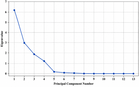
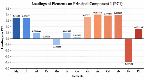
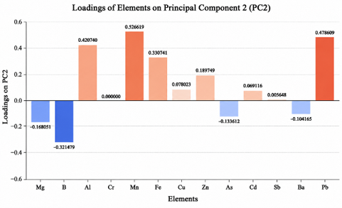
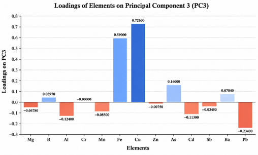
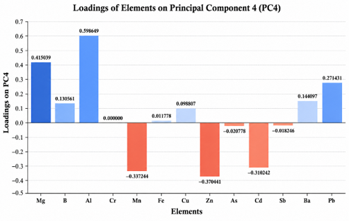
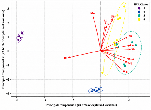
Principal component analysis was employed to identify the major sources of variability among heavy metals and to reduce data dimensionality (Figure 2). The first two principal components (PC1 and PC2) explained approximately 72.48% of the total variance, with PC1 accounting for 48.87% and PC2 accounting for 23.61%, as shown in Table 4. The principal component analysis biplot revealed clear separation among the monitoring stations and highlighted the metals contributing most strongly to spatial differentiation. Positive loadings along PC1 were mainly associated with Zn, Cd, As, Sb, Cu, Mg, and B, while PC2 was strongly influenced by Mn, Pb, Al, and Fe (Figure 3).
Figure 2. Principal component analysis of the first four principal components
(a)
(b)
(c)
(d)
The clustering pattern observed in the principal component analysis ordination indicated that several monitoring sectors share similar contamination signatures, whereas others exhibit markedly distinct geochemical profiles. The opposite position of Ba relative to most metals suggests a different geochemical behavior and potentially a different origin. Overall, principal component analysis demonstrated that the spatial variability of heavy metal concentrations is primarily governed by a limited set of discriminating elements, notably B, Zn, Mn, As, Cd, and Pb.
3.3 Hierarchical cluster analysis
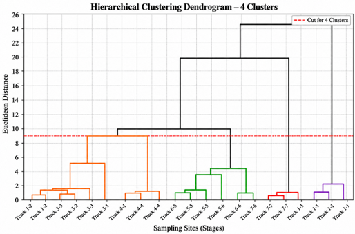
Hierarchical cluster analysis was performed using Euclidean distance and Ward’s linkage method to classify monitoring stations according to similarities in metal concentrations, The dendrogram (Figure 4) identified four major clusters, confirming the existence of significant spatial heterogeneity throughout the sub-basin, Cluster 1 grouped all stations from Track 1, which remained highly separated from the remaining stations, indicating a unique contamination profile, Clusters 2 and 3 were primarily composed of stations from Tracks 2, 3, 4, 5, and 6, suggesting moderate similarity in metal composition, Cluster 4 contained stations with the most distinct contamination characteristics, reflecting localized environmental conditions or specific pollution sources, The large linkage distances separating the clusters indicate substantial differences in metal concentrations among monitoring sectors, These results confirm that contamination is not uniformly distributed throughout the watershed but rather follows spatially structured patterns.
Table 4. Factor loadings, eigenvalues, and explained variance
|
Elements |
PC1 |
PC2 |
PC3 |
PC4 |
|
Mg |
0.34646 |
-0.168051 |
-4.78E−02 |
0.415039 |
|
B |
0.339172 |
-0.321479 |
3.97E−02 |
0.130561 |
|
Al |
0.084866 |
0.42074 |
-1.24E−01 |
0.598649 |
|
Cr |
0 |
0 |
-4.86E−17 |
0 |
|
Mn |
-0.101888 |
0.526619 |
-8.50E−02 |
-0.337244 |
|
Fe |
0.082592 |
0.330741 |
5.90E−01 |
0.011778 |
|
Cu |
0.020622 |
0.078023 |
7.26E−01 |
0.098807 |
|
Zn |
0.352221 |
0.189749 |
-7.50E−03 |
-0.370441 |
|
As |
0.391872 |
-0.133612 |
1.60E−01 |
-0.020778 |
|
Cd |
0.375297 |
0.069116 |
-1.13E−01 |
-0.310242 |
|
Sb |
0.385039 |
0.005648 |
-3.45E−02 |
-0.018246 |
|
Ba |
-0.387132 |
-0.104165 |
7.04E−02 |
0.144097 |
|
Pb |
0.153295 |
0.478609 |
-2.34E−01 |
0.271431 |
|
Eigenvalue |
6.157572 |
2.974543 |
1.91E+00 |
1.208944 |
|
Variance explained (%) |
48.869621 |
23.607481 |
1.51E+01 |
9.594797 |
|
Cumulative variance explained (%) |
48.869621 |
72.477102 |
8.76E+01 |
97.197018 |
Note: PC1: Principal component 1; PC2: Principal component 2; PC3: Principal component 3; PC4: Principal component 4.
Hierarchical cluster analysis using Ward’s method and Euclidean distance identified four major groups of monitoring stations. The cutoff distance of approximately 8.9 was selected based on the dendrogram structure, where a clear separation among four major clusters was observed.
Figure 4. Dendrogram of the hierarchical cluster analysis of the sampling stations, showing the classification into four groups
The hierarchical cluster analysis identified four main clusters of monitoring stations with distinct geochemical characteristics, The group corresponding to Track 1 showed the greatest separation from the rest of the stations, suggesting the influence of particular environmental conditions or specific sources of contamination, Tracks 5 and 6 formed a homogeneous cluster, indicating similarities in heavy metal concentrations and possible common sources of input, Meanwhile, Tracks 2, 3, and 4 were grouped into a single cluster, indicating a comparable chemical composition, albeit with some internal variability, The results obtained using hierarchical cluster analysis were consistent with the distribution observed in the principal component analysis, confirming the existence of distinct spatial patterns in the middle sub-basin of the Rímac River and supporting the presence of multiple processes controlling the distribution of heavy metals.
3.4 Multidimensional scaling
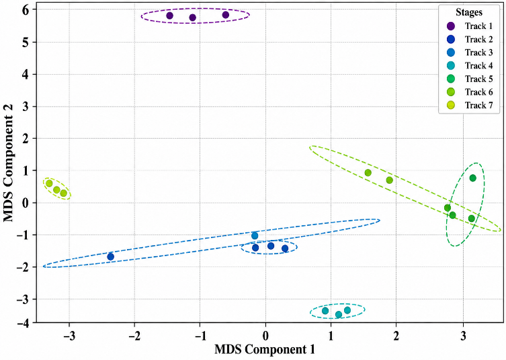
The multidimensional scaling analysis provided an alternative visualization of similarities among monitoring stations, The multidimensional scaling plot revealed a clear separation of the seven monitoring tracks based on their heavy metal profiles, Track 1 occupied an isolated position in the ordination space, suggesting a unique geochemical signature, Similarly, Track 4 appeared separated from the other groups, indicating distinct contamination conditions, Tracks 2 and 3 exhibited relatively close positions, reflecting similar metal concentration patterns, Likewise, Tracks 5 and 6 formed neighboring groups, suggesting shared contamination sources or hydrogeochemical conditions, Track 7 was clearly differentiated from all other sectors and displayed high internal homogeneity, The consistency between multidimensional scaling, principal component analysis, and hierarchical cluster analysis confirms the robustness of the spatial patterns identified in the dataset.
Figure 5. Biplot of the principal component analysis showing the classification of stations using hierarchical cluster analysis and the factor loadings for heavy elements
Figure 5 shows that PC1 = 48.87% on the X-axis and PC2 = 23.61% on the Y-axis, meaning that 48.87 + 23.61 = 72.48% of the total variability is explained by the first two components. The first two principal components explained 72.48% of the total variance in the data, indicating that the multivariate structure of heavy metal concentrations can be adequately represented in a two-dimensional space. This percentage exceeds the 70% threshold commonly accepted in environmental studies for interpretation.
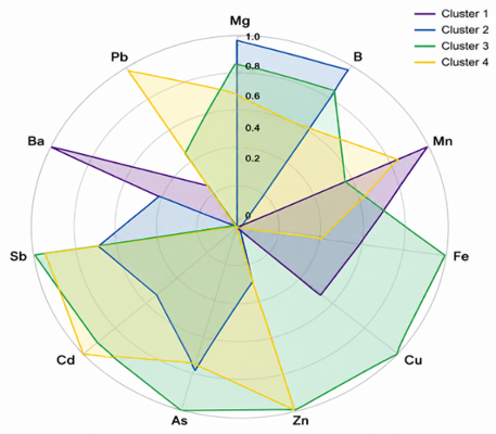
Multidimensional scaling analysis revealed a clear spatial segregation of the monitoring stations based on their heavy metal concentrations. The points belonging to each track formed compact, well-defined clusters, indicating high internal homogeneity within each sector. As shown in Figure 6, Track 1 and Track 4 showed the greatest separation from the rest of the groups, suggesting distinct geochemical conditions and possible specific sources of contamination. On the other hand, Tracks 2 and 3 exhibited considerable spatial proximity, as did Tracks 5 and 6, indicating similarities in their chemical profiles. The consistency observed among the multidimensional scaling, principal component analysis, and hierarchical cluster analysis results confirms the existence of robust spatial patterns in the distribution of heavy metals throughout the middle sub-basin of the Rímac River and supports the combined influence of geogenic and anthropogenic factors on the environmental quality of the river system. Figure 7 shows a comparison of standard metal profiles across clusters identified by hierarchical cluster analysis.
Figure 6. Multidimensional scaling (MDS) of the sampling stations and the groups identified through cluster analysis
Figure 7. Comparison of standard metal profiles across clusters identified by hierarchical cluster analysis
3.5 Analysis of variance
To validate the spatial differentiation identified through hierarchical cluster analysis, a one-way analysis of variance (ANOVA) was performed for each element. The results showed statistically significant differences among monitoring tracks for 12 of the 13 evaluated elements (p < 0.05), supporting the spatial heterogeneity observed in the multivariate analyses (Table 5).
The highest F-values were observed for Cd (F = 502.01, p < 0.001), followed by B (F = 432.79, p < 0.001), As (F = 315.62, p < 0.001), Al (F = 215.63, p < 0.001), and Mg (F = 199.44, p < 0.001). Zn (F = 77.96, p < 0.001), Mn (F = 68.61, p < 0.001), and Cu (F = 62.92, p < 0.001) also showed substantial differences among monitoring tracks. In contrast, ANOVA could not be computed for Cr because its concentration remained constant (0.0006 mg/L) across all monitoring stations, resulting in zero variance. These findings provide statistical support for the spatial heterogeneity identified through principal component analysis and hierarchical cluster analysis.
Table 5. Analysis of variance (ANOVA) statistics for the heavy metals analyzed
|
Elements |
Sum of Squares |
Mean Square |
F-Value |
p-Value |
|
Mg |
2.87E+01 |
4.78E+00 |
199.438332 |
9.76E-13 |
|
B |
5.09E-01 |
8.48E-02 |
432.793511 |
4.55E-15 |
|
Al |
1.11E-01 |
1.85E-02 |
215.62963 |
5.69E-13 |
|
Cr |
0 |
0 |
- |
- |
|
Mn |
9.10E-02 |
1.52E-02 |
68.609249 |
1.41E-09 |
|
Fe |
4.79E-02 |
7.99E-03 |
14.114728 |
3.19E-05 |
|
Cu |
2.81E-04 |
4.69E-05 |
62.918637 |
2.53E-09 |
|
Zn |
4.53E-01 |
7.56E-02 |
77.959913 |
5.98E-10 |
|
As |
8.80E-04 |
1.47E-04 |
315.616406 |
4.07E-14 |
|
Cd |
7.89E-06 |
1.31E-06 |
502.005455 |
1.62E-15 |
|
Sb |
8.01E-06 |
1.34E-06 |
14.381197 |
2.87E-05 |
|
Ba |
3.23E-04 |
5.38E-05 |
26.578335 |
6.94E-07 |
|
Pb |
2.07E-03 |
3.45E-04 |
25.012934 |
1.02E-06 |
Note: ANOVA was not computed for Cr because its concentration remained constant (0.0006 mg/L) across all monitoring stations, resulting in zero variance.
3.6 Random forest classification
Random forest was applied to identify the metals most relevant for discriminating monitoring sectors. The model achieved accuracy = 81%, macro-precision = 0.83, macro-recall = 0.81, and macro-F1 score = 0.79. These results indicate strong classification performance considering the small sample size and the seven monitoring sectors. Table 6 shows the most influential metals identified by random forest.
Moderate contributions were observed for Cd, Zn, As, Cu, and Al. The model assigned zero importance to Cr, reinforcing previous findings that chromium does not contribute to spatial differentiation within the study area. The confusion matrix showed that Classes 0 and 3 were perfectly classified (F1-score = 1.00), while Class 2 exhibited the lowest performance (F1-score = 0.50), indicating partial overlap with neighboring groups.
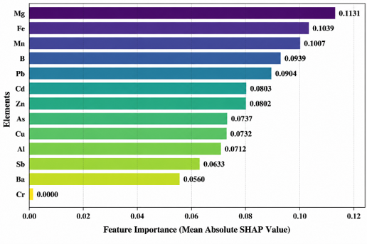
The random forest model was used to identify the metals with the greatest ability to spatially distinguish monitoring sites in the middle subbasin of the Rímac River, The results in Figure 8 showed that Mg was the most influential variable, with a relative importance of 0.1131 (11.31%), followed by Fe at 0.1039 (10.39%), Mn at 0.1007 (10.07%), B at 0.0939 (9.39%), and Pb at 0.0904 (9.04%), Together, these five elements accounted for 50.20% of the model’s total predictive power, A second significant group consisted of Cd (8.03%), Zn (8.02%), As (7.37%), Cu (7.32%), and Al (7.12%), all of which also contributed significantly to the differentiation of the monitoring stations, On the other hand, Sb (6.33%) and Ba (5.60%) made moderate contributions to the classification process, Cr had a relative importance of zero, indicating that this metal did not provide additional information for the spatial discrimination of the evaluated monitoring sites, This result suggests a relatively homogeneous distribution of Cr in the sub-basin or low variability among the analyzed stations.
Table 6. Importance of heavy elements according to the random forest model
|
Elements |
Importance |
|
Mg |
0.1131 |
|
Fe |
0.1039 |
|
Mn |
0.1007 |
|
B |
0.0939 |
|
Pb |
0.0904 |
|
Cd |
0.0803 |
|
Zn |
0.0802 |
|
As |
0.0737 |
|
Cu |
0.0732 |
|
Al |
0.0712 |
|
Sb |
0.0633 |
|
Ba |
0.0560 |
|
Cr |
0.0000 |
Figure 8. Ranking the importance of variables (heavy metals) using the random forest model
The high importance of Mg, Fe, and Mn suggests that the spatial differences observed in the watershed are strongly influenced by geological factors and weathering processes of the parent materials present in the study area, These elements are typically associated with the natural mineralogical composition of the rocks and sediments in the watershed, The significance of Pb, Cd, As, Cu, and Zn indicates that these metals are important markers of anthropogenic pollution in the middle Rímac River basin, The simultaneous presence of these elements is often linked to mining, metallurgical, and industrial activities historically carried out in the area, which have been reported as one of the main sources of pollution in the basin’s water resources, Boron exhibited a high relative importance (9.39%), making it the fourth most significant metal in the model, This pattern suggests that its spatial distribution contributes significantly to the differentiation among monitoring stations and could be associated with both natural geological processes and inputs from agricultural activities or industrial discharges,
3.7 Extreme gradient boosting classification and variable importance
The XGBoost model was applied as a complementary supervised-learning approach to classify the spatial groups identified for the monitoring stations. The model achieved an overall accuracy of 0.76, with macro-averaged precision, recall, and F1-score values of 0.77, 0.76, and 0.76, respectively. These results indicate that the elemental concentration profiles contain sufficient discriminatory information to distinguish most of the spatial groups, although model performance should be interpreted cautiously given the limited sample size (n = 21).
Variable-importance analysis showed that Al had the highest relative contribution (11.94%), followed by Cd (9.67%), Fe (9.50%), Sb (9.50%), B (9.40%), Pb (9.13%), and As (8.90%). Cu, Mg, Zn, and Mn showed intermediate contributions, whereas Ba had relatively low importance and Cr contributed no measurable discriminatory information in the fitted model (Table 7). The importance values sum to approximately 100%, with a minor difference attributable to rounding.
Table 7. Variable importance in the extreme gradient boosting (XGBoost) model
|
Element |
Importance |
|
Al |
11.94 |
|
Cd |
9.67 |
|
Fe |
9.50 |
|
Sb |
9.50 |
|
B |
9.40 |
|
Pb |
9.13 |
|
As |
8.90 |
|
Cu |
7.87 |
|
Mg |
7.04 |
|
Zn |
6.82 |
|
Mn |
6.44 |
|
Ba |
3.80 |
|
Cr |
0.00 |
The variable-importance pattern suggests that spatial classification was influenced by both elements commonly associated with geological background (particularly Al and Fe) and elements that may also reflect anthropogenic inputs, including Cd, Pb, As, Cu, and Sb. However, XGBoost importance scores quantify predictive contribution rather than source attribution; therefore, potential geogenic or anthropogenic origins should be interpreted jointly with the contamination factors, spatial distribution, PCA loadings, and hydrogeochemical context.
At the class level, Classes 0 and 3 were classified perfectly (precision = recall = F1-score = 1.00), while Class 6 showed high sensitivity (recall = 1.00). Class 4 had the lowest performance (precision = 0.50, recall = 0.33, and F1-score = 0.40), indicating greater overlap with the elemental profiles of other spatial groups (Table 8).
Table 8. Classification performance of the extreme gradient boosting (XGBoost) model
|
Class |
Precision |
Recall |
F1-score |
Support |
|
0 |
1 |
1 |
1 |
3 |
|
1 |
1 |
0.67 |
0.8 |
3 |
|
2 |
0.67 |
0.67 |
0.67 |
3 |
|
3 |
1 |
1 |
1 |
3 |
|
4 |
0.5 |
0.33 |
0.4 |
3 |
|
5 |
0.5 |
0.67 |
0.57 |
3 |
|
6 |
0.75 |
1 |
0.86 |
3 |
|
Macro-average |
0.77 |
0.76 |
0.76 |
21 |
|
Weighted average |
0.77 |
0.76 |
0.76 |
21 |
For comparison, Random Forest yielded numerically higher evaluation metrics than XGBoost, with accuracy values of 0.81 and 0.76, respectively (Table 9). The same pattern was observed for precision, recall, and F1-score. Given the small dataset, these differences are reported descriptively and should not be interpreted as conclusive evidence that one algorithm is generally superior to the other.
Table 9. Performance comparison of Random Forest and extreme gradient boosting (XGBoost) models
|
Metric |
Random Forest |
XGBoost |
|
Accuracy |
0.81 |
0.76 |
|
Precision |
0.83 |
0.77 |
|
Recall |
0.81 |
0.76 |
|
F1-score |
0.79 |
0.76 |
Overall, the XGBoost results were broadly consistent with the multivariate and Random Forest analyses in identifying structured spatial variation in elemental concentrations. Elements such as B, As, Cd, Pb, and Cu repeatedly contributed to the differentiation of monitoring stations across complementary analytical approaches. This convergence strengthens the interpretation of spatial heterogeneity in the middle Rímac River sub-basin, while the limited sample size warrants cautious interpretation of predictive performance and variable-importance estimates.
Given the limited sample size (n = 21), these predictive metrics should be interpreted as exploratory and would benefit from validation using a larger independent dataset.
4.1 Spatial variability of heavy metal contamination
The contamination factor analysis revealed substantial spatial variability in the middle Rímac River sub-basin, with B, Zn, Mn, As, and Cd exhibiting the highest contamination levels. These findings suggest the coexistence of multiple contamination sources, including mining activities, geological weathering, industrial discharges, and urban runoff. The elevated contamination factors observed for As and Cd are consistent with recent studies conducted in mining-impacted watersheds, where these potentially toxic elements have been associated with mining-related contamination and the mobilization of metals from mineralized materials and mine wastes [27]. Similarly, Zn and Pb are commonly reported among the potentially toxic elements enriched in river sediments affected by mining and metallurgical activities, reflecting the influence of mine tailings, smelting, and other anthropogenic sources [28]. The Rímac River basin has historically been influenced by intensive mining operations in the central Andes of Peru, which likely contribute to the observed enrichment of toxic metals. The high contamination factors found for B and Mn may also reflect lithological contributions from volcanic and sedimentary formations, indicating that both geogenic and anthropogenic processes influence water quality in the study area.
4.2 Chemometric identification of contamination patterns
The application of random forest and XGBoost provided additional insights into the metals responsible for spatial differentiation. Random forest identified Mg, Fe, Mn, B, and Pb as the most influential predictors, while XGBoost highlighted Al, Cd, Fe, Sb, and B. Despite differences in variable ranking, both models identified B, Fe, and Pb among the influential discriminating variables, while Cd, Mn, As, and other elements showed model-dependent contributions. The convergence of these findings strengthens the interpretation that these metals play a key role in defining contamination patterns across the sub-basin. Previous studies have demonstrated the effectiveness of random forest for identifying environmental drivers and classifying pollution sources due to its robustness against multicollinearity and nonlinear relationships [29, 30]. Similarly, XGBoost has emerged as one of the most powerful machine learning algorithms for environmental applications because of its ability to capture complex interactions among variables while maintaining high predictive performance [31]. The fact that chromium consistently exhibited zero importance in both models further supports the statistical evidence obtained from analysis of variance and descriptive analyses, confirming its negligible contribution to spatial variability.
4.3 Statistical validation through analysis of variance
The analysis of variance results demonstrated significant differences among monitoring tracks for 12 of the 13 evaluated elements. Cd, B, As, Al, and Mg exhibited the highest F-statistics, indicating pronounced spatial differentiation.
These findings support the multivariate analyses and confirm that elemental concentrations exhibit marked spatial heterogeneity across the study area. In contrast, Cr showed no measurable variability across the monitoring stations, consistent with its constant concentration. The statistical significance observed in the analysis of variance reinforces the spatial differentiation among monitoring tracks and supports the non-uniform distribution of elemental concentrations across the study area. Similar conclusions have been reported, indicating that elements associated with lithogenic sources tend to display lower spatial variability than metals derived from human activities [32].
4.4 Machine learning interpretation of heavy metal drivers
The application of random forest and XGBoost provided additional insights into the metals responsible for spatial differentiation. Random forest identified Mg, Fe, Mn, B, and Pb as the most influential predictors, while XGBoost highlighted Al, Cd, Fe, Sb, and B. Despite differences in variable ranking, both models consistently identified B, Cd, Pb, Fe, and Mn as important discriminating variables. The convergence of these findings strengthens the interpretation that these metals play a key role in defining contamination patterns across the sub-basin. Previous studies have demonstrated the effectiveness of random forest for identifying environmental drivers and classifying pollution sources due to its robustness against multicollinearity and nonlinear relationships [33, 34]. Similarly, XGBoost has emerged as one of the most powerful machine learning algorithms for environmental applications because of its ability to capture complex interactions among variables while maintaining high predictive performance [35]. The fact that chromium consistently exhibited zero importance in both models further supports the statistical evidence obtained from analysis of variance and descriptive analyses, confirming its negligible contribution to spatial variability.
4.5 Contribution of explainable machine learning to environmental assessment
One of the main methodological contributions of this study is the integration of traditional chemometric techniques with explainable machine learning approaches. Environmental studies have traditionally relied on principal component analysis and clustering methods to identify contamination sources. However, these methods do not always provide clear information regarding the relative importance of individual variables. By incorporating random forest and XGBoost, the present study was able to quantify the relative contribution of each metal to the observed spatial classification patterns. Recent research has emphasized the growing importance of explainable artificial intelligence in environmental sciences, particularly for improving transparency and supporting evidence-based decision-making [36, 37]. The integration of chemometrics and explainable machine learning therefore provides a more comprehensive framework for identifying contamination sources, understanding spatial variability, and prioritizing remediation efforts.
4.6 Environmental implications for the Rímac River basin
The combined evidence obtained from elemental concentrations, multivariate statistics, and machine learning indicates that B, Zn, Mn, As, Cd, and Pb are important elements for understanding spatial variability in the middle Rímac River sub-basin. Several of these elements, particularly As, Cd, and Pb, are recognized as environmentally persistent contaminants that may pose ecological and human-health concerns depending on concentration, exposure, and environmental conditions [38]. Similar concerns have been reported in mining-affected river sediments from the Peruvian Central Highlands. The spatial patterns identified in this study support the need for continued monitoring of sectors influenced by mining and other anthropogenic activities. The proposed analytical framework may also be applied to other Andean watersheds experiencing similar environmental pressures.
The present study integrated chemometric techniques and explainable machine learning methods to investigate the spatial patterns and potential sources of heavy metal contamination in the middle Rímac River sub-basin, Peru. Based on the obtained results, the following conclusions can be drawn:
(a) The measured concentrations of the 13 elements showed clear spatial variation across the study area. B, Zn, Mn, As, Cd, and Pb displayed marked differences among monitoring sectors, indicating that these elements are particularly relevant for characterizing the environmental variability of the middle Rímac River sub-basin.
(b) The chemometric analyses, including principal component analysis, hierarchical cluster analysis, and multidimensional scaling, consistently identified well-defined spatial patterns among monitoring stations. These methods demonstrated that heavy metal contamination is not uniformly distributed throughout the watershed but instead exhibits marked spatial heterogeneity. The clustering structure revealed the existence of sectors with distinct geochemical signatures, suggesting the influence of multiple contamination sources and environmental processes.
(c) The analysis of variance results demonstrated significant differences among monitoring tracks for 12 of the 13 evaluated elements (p < 0.05). Cd, B, As, Al, and Mg exhibited the highest F-statistics, indicating pronounced spatial differentiation. Cr was not subjected to ANOVA because its concentration remained constant across all monitoring stations, resulting in zero variance.
(d) The machine learning models successfully classified monitoring sectors based on heavy metal concentrations. Random forest achieved the best overall performance, with an accuracy of 81%, while XGBoost reached an accuracy of 76%. The satisfactory predictive performance of both algorithms confirms that the spatial variability of heavy metals follows identifiable patterns that can be effectively modeled using advanced data-driven approaches.
(e) The feature importance analyses performed through random forest and XGBoost showed partially convergent importance patterns, with B, Fe, and Pb identified as influential by both models, while Cd, Mn, As, and other elements displayed model-dependent contributions to spatial discrimination. Furthermore, Cr exhibited negligible importance in all statistical and machine learning analyses, indicating a homogeneous distribution and limited contribution to spatial discrimination.
(f) The integration of chemometric methods and explainable machine learning provided complementary and mutually reinforcing evidence regarding the sources and spatial distribution of contamination. The convergence of results obtained from principal component analysis, hierarchical cluster analysis, multidimensional scaling, analysis of variance, random forest, and XGBoost strengthens the reliability of the findings and demonstrates the robustness of the proposed analytical framework.
(g) The observed contamination patterns suggest the combined influence of geogenic processes and anthropogenic activities, particularly mining and industrial operations historically developed within the Rímac River basin. The elevated contamination levels detected for As, Cd, Pb, Zn, and Cu indicate the need for continuous environmental monitoring and targeted management strategies aimed at reducing pollutant inputs and protecting aquatic ecosystems and human health.
(h) Finally, the proposed framework represents an innovative approach for environmental assessment by combining traditional multivariate statistics with explainable artificial intelligence techniques. This methodology can be applied to other mining-impacted watersheds worldwide to support pollution source identification, environmental monitoring programs, and evidence-based watershed management.
This work was supported by Universidad Peruana Unión (UPeU) through the internal research competition PID FID_01-2025-07, “Research Projects in Basic Sciences,” approved under Resolution N° 0300-A-2025/UPeU/FIA/CU, as well as by APC funding.
[1] Nazir, A., Khan, M.A., Ghosh, P. (2022). Assessment of variations in metal concentrations of the Ganges River water by using multivariate statistical techniques. Limnologica, 95: 125989. https://doi.org/10.1016/j.limno.2022.125989
[2] Vareda, J.P., Valente, A.J., Durães, L. (2019). Assessment of heavy metal pollution from anthropogenic activities and remediation strategies: A review. Journal of Environmental Management, 246: 101-118. https://doi.org/10.1016/J.JENVMAN.2019.05.126
[3] Digué, T.M., Bibriven, L.R., Bertrand, N.G. (2026). Assessment of heavy metal contamination of fish (Tilapia niloticus and Synodontis schall) from the Chari and Logone rivers near the city of N'Djamena in Chad. Next Research, 7: 101476. https://doi.org/10.1016/j.nexres.2026.101476
[4] Custodio, M., Peñaloza, R., De la Cruz, H. (2025). Risk assessment of heavy metals and pharmaceutically active compounds in river water from the central region of Peru. Environmental Challenges, 19: 101152. https://doi.org/10.1016/j.envc.2025.101152
[5] Ccanccapa-Cartagena, A., Chavez-Gonzales, F.D., Paredes, B., et al. (2023). Seasonal differences in trace metal concentrations in the major rivers of the hyper-arid southwestern Andes basins of Peru. Journal of Environmental Management, 344: 118493. https://doi.org/10.1016/j.jenvman.2023.118493
[6] Piwowarska, D., Kiedrzyńska, E., Jaszczyszyn, K. (2024). A global perspective on the nature and fate of heavy metals polluting water ecosystems, and their impact and remediation. Critical Reviews in Environmental Science and Technology, 54(19): 1436-1458. https://doi.org/10.1080/10643389.2024.2317112
[7] Putuhena, D.J. (2025). Global water scarcity assessment: Remote sensing evaluation of climate change impacts on freshwater resources. International Journal of Environmental Impacts, 8(5): 907-920. https://doi.org/10.56578/ijei080507
[8] Salinas-Castro, A., Santillán-Fernández, A., Rau, P., Bourrel, L. (2026). Assessing Shrub and grassland degradation portfolios as benchmarks for potential water quantity benefits: Application of the RIOS and SWAT model to Rimac Basin, Peru. Land, 15(4): 638. https://doi.org/10.3390/land15040638
[9] Samaniego, T., La Torre, R., Orjeda, G., Ramirez, J.L. (2025). Lima megacity’s influence on aquatic microbial communities in the Rímac River: Dominance over spatial and seasonal variations. Microbial Ecology, 88(1): 57. https://doi.org/10.1007/s00248-025-02558-5
[10] Castro-Castro, G.C., Ardila-Pereira, L.C., Orozco-Muñoz, Y.S., Sepulveda-Lazaro, E.E., Molina-Castro, C.E. (2018). Risk factors associated with musculoskeletal disorders in a refrigerator manufacturing company. Revista de Salud Publica, 20(2): 182-188. https://doi.org/10.15446/rsap.v20n2.57015
[11] Dominguez-Lara, S., Merino-Soto, C., Torres-Villalobos, G. (2022). Structural analysis and reliability of the Perceived Stress Scale in nursing professionals from Peru. Enfermería Clínica, 32(3): 152-160. https://doi.org/10.1016/J.ENFCLI.2022.01.003
[12] Custodio, M., Peñaloza, R., Chanamé, F., Hinostroza-Martínez, J.L., De la Cruz, H. (2021). Water quality dynamics of the Cunas River in rural and urban areas in the central region of Peru. Egyptian Journal of Aquatic Research, 47(3): 253-259. https://doi.org/10.1016/j.ejar.2021.05.006
[13] Cesar Minga, J., Elorza, F.J., Rodriguez, R., Iglesias, A., Esenarro, D. (2023). Assessment of water resources pollution associated with mining activities in the Parac subbasin of the Rimac River. Water, 15(5): 965. https://doi.org/10.3390/w15050965
[14] Crespo, M.A.D., Cadillo, S.R.B., Baldeon, S.A.G., Esperilla, N.S.D., Malca, U.F.G. (2023). Variation in the concentration of heavy metals due to rains and floods in the Rimac river basin, Lima-Peru. In Proceedings of the LACCEI International Multi-conference for Engineering, Education and Technology. https://doi.org/10.18687/laccei2023.1.1.1061
[15] Ccanccapa-Cartagena, A., Paredes, B., Vera, C., et al. (2021). Occurrence and probabilistic health risk assessment (PRA) of dissolved metals in surface water sources in Southern Peru. Environmental Advances, 5: 100102. https://doi.org/10.1016/j.envadv.2021.100102
[16] Mori Sosa, L.J.P., Morales Cabrera, D.U., Florez Ponce De León, W.D., Hinojosa Ramos, E.A., Torres Ventura, A.Y. (2025). Study of arsenic contamination in the Caplina basin, Tacna, Peru: Arsenite and arsenate analysis using inductively coupled plasma mass spectrometry and high-performance liquid chromatography. Sustainability, 17(2): 611. https://doi.org/10.3390/su17020611
[17] Islam, M.S., Al-Bakky, A., Islam, A.R.M.T., et al. (2026). Ecological risk and source apportionment of heavy metals in riparian soil and sediment of an urban river in a developing country. Scientific Reports, 16(1): 4856. https://doi.org/10.1038/s41598-026-35479-5
[18] Rahman, M.S., Ahmed, Z., Seefat, S.M., et al. (2022). Assessment of heavy metal contamination in sediment at the newly established tannery industrial Estate in Bangladesh: A case study. Environmental Chemistry and Ecotoxicology, 4: 1-12. https://doi.org/10.1016/j.enceco.2021.10.001
[19] Wilson, I., Peters, A., Merrington, G., et al. (2024). Practical estimation and use of natural background concentrations in surface waters for nickel in Europe. Integrated Environmental Assessment and Management, 20(6): 2128-2141. https://doi.org/10.1002/ieam.4988
[20] Kumar, H., Sarkar, A., Singh, U., Singh, N., Jain, S., Dutta, A. (2025). Water chemistry and estimation of local geochemical background values of elements in headwater streams of Ken–Betwa catchment of Yamuna River, India. Environmental Earth Sciences, 84(2): 51. https://doi.org/10.1007/s12665-024-12059-2
[21] Moreno-Aguirre, S.B., Vértiz-Osores, J.J., Paredes-Espinal, C.E., et al. (2024). Ecological risk of metals in Andean water resources: A framework for early environmental assessment of mining projects in Peru. Heliyon, 10(9): e30739. https://doi.org/10.1016/j.heliyon.2024.e30739
[22] Jin, X., Wu, Q., Peñuelas, J., et al. (2025). Climate and anthropogenic activities control the concentrations of copper, zinc, cadmium and chromium in global inland waters. Communications Earth & Environment, 6(1): 520. https://doi.org/10.1038/s43247-025-02508-6
[23] Quispe-Zuniga, M. R., Santos, F., Callo-Concha, D., Greve, K. (2019). Impact of heavy metals on community farming activities in the Central Peruvian Andes. Minerals, 9(10): 647. https://doi.org/10.3390/min9100647
[24] McClain, C.N., Maher, K. (2016). Chromium fluxes and speciation in ultramafic catchments and global rivers. Chemical Geology, 426: 135-157. https://doi.org/10.1016/j.chemgeo.2016.01.021
[25] Amarante, R.T., Marques, E.D., Ruchkys, Ú.A., et al. (2025). Geochemical baseline and multivariate analysis of potentially toxic elements in stream sediments of the Vazante Zinc district, Minas Gerais, Brazil. Frontiers in Environmental Science, 13: 1684687. https://doi.org/10.3389/fenvs.2025.1684687
[26] Liu, N., Li, X., Chen, P., Yuan, W., Wang, D., Wang, X. (2025). Climate and vegetation controlling accumulation and translocation of heavy metals in water tower regions of Qinghai-Tibet Plateau. Journal of Hazardous Materials, 484: 136752. https://doi.org/10.1016/j.jhazmat.2024.136752
[27] Joe, D.J., Choi, M.S., Lee, J.H., Kim, C.K. (2025). Identifying mining and smelting contributions to metal contamination in lake and river sediments, South Korea. Environmental Earth Sciences, 84(15): 430. https://doi.org/10.1007/s12665-025-12439-2
[28] Khan, K., Younas, M., Yaseen, M., et al. (2025). Heavy metals pollution in riverine sediments: Distribution, source, and environmental implications. Environmental Monitoring and Assessment, 197(3): 225. https://doi.org/10.1007/s10661-025-13623-4
[29] Liu, T., Wang, M., Wang, M., et al. (2025). Identification of the primary pollution sources and dominant influencing factors of soil heavy metals using a random forest model optimized by genetic algorithm coupled with GeoDetector. Ecotoxicology and Environmental Safety, 290: 117731. https://doi.org/10.1016/j.ecoenv.2025.117731
[30] Qin, Z., Peng, Q., Jin, C., et al. (2025). Geographically weighted random forest fusing multi-source environmental covariates for spatial prediction of soil heavy metals. Environmental Pollution, 385: 127135. https://doi.org/10.1016/j.envpol.2025.127135
[31] Li, X., Gu, H., Tang, R., et al. (2025). A fusion XGBoost approach for large-scale monitoring of soil heavy metal in farmland using hyperspectral imagery. Agronomy, 15(3): 676. https://doi.org/10.3390/agronomy15030676
[32] Eti, S.A., Islam, M.S., Shourove, J.H., et al. (2023). Assessment of heavy metals migrated from food contact plastic packaging: Bangladesh perspective. Heliyon, 9(9): e19667. https://doi.org/10.1016/j.heliyon.2023.e19667
[33] Wang, J., Deng, Y., Huang, Z., Li, D.A., Zhang, X. (2025). Identification of driving factors for heavy metals and polycyclic aromatic hydrocarbons pollution in agricultural soils using interpretable machine learning. Science of the Total Environment, 960: 178384. https://doi.org/10.1016/j.scitotenv.2025.178384
[34] Proshad, R., Asha, S.A.A., Tan, R., et al. (2025). Machine learning models with innovative outlier detection techniques for predicting heavy metal contamination in soils. Journal of Hazardous Materials, 481: 136536. https://doi.org/10.1016/j.jhazmat.2024.136536
[35] Jain, S., Bawa, A., Mendoza, K., et al. (2025). Enhancing prediction and inference of daily in-stream nutrient and sediment concentrations using an extreme gradient boosting based water quality estimation tool-XGBest. Science of the Total Environment, 963: 178517. https://doi.org/10.1016/j.scitotenv.2025.178517
[36] Yan, Y., Yang, Y. (2025). Revealing the synergistic spatial effects in soil heavy metal pollution with explainable machine learning models. Journal of Hazardous Materials, 482: 136578. https://doi.org/10.1016/j.jhazmat.2024.136578
[37] Schiller, J., Stiller, S., Ryo, M. (2025). Artificial intelligence in environmental and Earth system sciences: Explainability and trustworthiness. Artificial Intelligence Review, 58(10): 316. https://doi.org/10.1007/s10462-025-11165-2
[38] Jomova, K., Alomar, S.Y., Nepovimova, E., Kuca, K., Valko, M. (2025). Heavy metals: Toxicity and human health effects. Archives of Toxicology, 99(1): 153-209. https://doi.org/10.1007/s00204-024-03903-2