Syafrudin | Sudarno | Mochamad Arief Budihardjo* | Alain Sofia | Azahra Septiana Azizah
© 2026 The authors. This article is published by IIETA and is licensed under the CC BY 4.0 license (http://creativecommons.org/licenses/by/4.0/).
OPEN ACCESS
This study investigates sediment transport dynamics and lead (Pb) contamination in the Banjir Kanal Timur estuarine system and the Lamper River, Central Java, Indonesia. Sediment samples were collected as bed load and suspended load following ISO 5667-12:2017 and ISO 5667-17:2000 standards. Laboratory analyses included granulometric and gravimetric analyses, as well as heavy-metal determination using Atomic Absorption Spectrophotometry (AAS). River discharge was measured based on SNI 03-2414-1991, while heavy-metal extraction and quantification followed standardized SNI procedures. Sediment transport rates were calculated using empirical formulations incorporating hydraulic and geomorphological parameters. The results show that sand was the dominant sediment fraction at most stations, ranging from 38.51% to 61.20%, while silt ranged from 31.29% to approximately 59.50% and clay ranged from 0.76% to 20.21%. Lead (Pb) concentrations ranged from 15.09 to 21.91 mg/kg and remained below the applied sediment-quality guideline threshold. However, Geoaccumulation Index (Igeo) values of 4.65–5.19 indicated heavily to extremely contaminated conditions, while Enrichment Factor (EF) values of 1.61–2.34 suggested minor anthropogenic enrichment. Spatial variability in sediment transport was influenced by discharge, channel morphology, and tidal dynamics, with the estuarine stations generally exhibiting higher transport rates than the upstream station. These findings demonstrate the influence of urbanization and anthropogenic activities on sediment quality and distribution patterns in tropical river estuaries.
sediment transport, heavy-metal contamination, lead, estuarine system, Geo-accumulation Index, river discharge, SNI standards
Sediment transport refers to the movement of particulate matter driven by flowing water in rivers and other aquatic systems [1]. Sediments, which are primarily composed of sand and mineral particles, accumulate and initiate transport processes that contribute to riverbed formation through aggradation and the development of deltaic environments [2, 3]. Sedimentation is the settling process through which particles in the water column are deposited onto the riverbed, whereas sediment transport encompasses the processes that keep these particles in suspension or motion. The interaction between these mechanisms is fundamental to river-system analysis, particularly for understanding sediment distribution, habitat conditions, and channel morphology [4, 5]. These processes also influence water quality, riverbank stability, and streambed structure because sediments transport essential nutrients, organic matter, and minerals that sustain aquatic ecosystems. However, sediments can also act as carriers of pollutants, including heavy metals originating from agricultural runoff, industrial discharge, and urban wastewater [6, 7]. The presence of such contaminants degrades water quality and poses significant environmental risks to aquatic life. In urban rivers, pollution is further intensified by industrial activities and residential development, which introduce anthropogenic contaminants into sediments. Consequently, the physical and chemical alteration of sediments contributes to water-quality deterioration, environmental degradation, biodiversity loss, and potential risks to human health. In Southeast Asia, urban river conditions have deteriorated significantly due to increased sediment loads carrying hazardous substances [8, 9], highlighting the urgent need for comprehensive sediment-management strategies to control contaminant transport and mitigate river-basin pollution.
In Indonesia, several rivers, including those in Semarang, Central Java, are experiencing substantial heavy-metal contamination [10, 11]. Rivers that traditionally function as channels for water conveyance are increasingly being used as disposal sites for industrial effluents and domestic waste. This practice has resulted in the accumulation of contaminated sediments, particularly near river mouths, which generates adverse environmental impacts. Estuarine zones play a critical role as transitional areas that influence overall river-water quality [12]. Among various pollutants, lead (Pb) is one of the most commonly detected heavy metals in urban river systems and poses serious risks to both human health and aquatic ecosystems [13]. The primary sources of lead contamination include industrial activities and vehicular emissions, especially from the historical use of leaded gasoline before its phase-out in Indonesia in 2006 [14].
Although policies banning the use of leaded fuel have been implemented, lead residues persist in sediments and soils because of their stable and non-biodegradable characteristics. Hydrological processes within river systems further facilitate the redistribution of these contaminants, increasing risks to ecosystems and communities in estuarine areas. Industrial activities, such as automotive workshops, textile production, and food processing, also continue to contribute to environmental lead pollution through direct discharge [15]. Numerous studies have examined the distribution and impacts of heavy metals on water quality. For example, Wu et al. [16] assessed potential health risks associated with heavy-metal exposure, while Zhao et al. [17] investigated the influence of heavy metals on microbial communities and demonstrated their disruption of nutrient cycling and aquatic ecosystem balance. In addition, Sheng et al. [18] highlighted the significant role of microbial activity in sediments in regulating nutrient dynamics and pollutant degradation.
Despite these findings, most previous studies have focused primarily on heavy-metal contamination in sediments without considering sediment transport dynamics along river systems. Existing research also tends to emphasize the relationship between microbial activity and heavy-metal pollution, while overlooking the potential use of heavy metals as indicators of river-water quality. A critical research gap, therefore, remains in the integrated analysis of sediment transport processes, heavy-metal distribution, and tidal influences within tropical urban estuarine systems, particularly in the Indonesian context. Accordingly, this study aims to analyze the transport of lead (Pb) in Indonesian rivers, with particular emphasis on its movement through sediment pathways. The analysis is supported by sediment characterization, including both bed load and suspended load, across several monitoring stations. The novelty of this research lies in combining sediment transport quantification, Pb contamination assessment using multiple indices (Geoaccumulation Index (Igeo), Contamination Factor (Cf), and EF), and tidal-dynamic considerations within a single integrated framework. This study is expected to provide insights into sedimentation characteristics, transport velocity, and their implications for river-water quality, ultimately contributing to the development of effective pollution-control strategies to protect water resources and public health in urban environments.
2.1 Study area
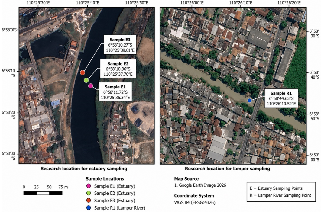
The study was conducted between June and August 2024 at two primary research locations: the Banjir Kanal Timur estuary and the Lamper River (see Figure 1 and Figure 2). Sampling in the estuarine area was conducted at three observation stations: Station E1 (6°57'6.81''S, 110°26'25.48''E), Station E2 (6°57'6.63''S, 110°26'25.06''E), and Station E3 (6°57'6.44''S, 110°26'24.60''E). In addition, one sampling point was established in the midstream section of the Lamper River, namely Station L (7°0'6.48"S, 110°26'39.20"E). Discharge measurements were conducted at the Banjir Kanal Timur Bridge, located approximately 5.06 km upstream from the estuary at 6°59'46.17"S and 110°26'20.91"E. This location was selected because of its hydrological stability, as it is not influenced by tidal fluctuations, thereby ensuring more reliable data. The site also offers practical advantages, including ease of access and a relatively shallow river profile, which facilitates more efficient sampling by minimizing constraints related to depth variability and tidal interference.
Figure 1. Research location for the estuary and Lamper River sampling
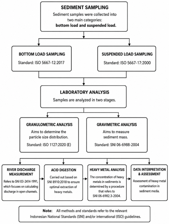
Figure 2. Flowchart of the data collection method
The Banjir Kanal Timur River primarily functions as a receiving body for runoff generated from various anthropogenic activities, including industrial, residential, and commercial sources. These characteristics formed the basis for its selection as the main study site. The river is highly suitable for investigating sediment transport and contaminant dynamics because of its significant sediment accumulation and high susceptibility to heavy-metal pollution. The Lamper River, as a tributary of the Banjir Kanal Timur, was also included to assess upstream flow contributions and compare pollution levels between interconnected river segments. Together, these two locations provide an integrated study area that enables a comprehensive analysis of sediment transport processes and pollution distribution along different sections of the river system in Indonesia.
2.2 Data collection method
A total of 12 independent sediment samples were collected over three months, from June to August 2024. Sampling was conducted at four points each month: three estuarine stations (E1, E2, and E3) and one upstream station in the Lamper River (L). Sediment samples were classified into two main categories: bed load and suspended load. Bed-load sampling followed ISO 5667-12:2017, while suspended-load sampling followed the procedures specified in ISO 5667-17:2000. All samples were immediately stored in acid-washed polyethylene containers, preserved at 4 ℃ in a cool box, and transported to the laboratory within 12 hours for further analysis.
For granulometric analysis, dried samples (105 ℃ for 24 hours) were first separated using a sieve shaker with mesh sizes ranging from 4.75 mm to 0.063 mm to obtain the sand fraction. The finer fraction (<0.063 mm), containing silt and clay, was further analyzed using the pipette method based on Stokes’ law, following ISO 1127:2020 (E). Gravimetric analysis was used to quantify sediment mass with reference to SNI 06-69398-2004. River discharge measurements were conducted based on SNI 03-2414-1991. Discharge was measured at a single representative point located approximately 5.06 km upstream of the estuary, at the Banjir Kanal Timur Bridge, which is not influenced by tidal backwater. For estuarine stations, discharge was assumed to be equal to this upstream value because no major tributaries occur between the measurement point and the sampling locations. However, the calculated transport rates are presented as estimates based on representative discharge rather than station-specific measured loads. Acid digestion was conducted according to SNI 8910:2021 to ensure optimal extraction of heavy metals from the samples. The concentration of Pb in the sediments was then determined using procedures outlined in SNI 06-6992.3-2004.
2.3 Laboratory analysis of sediment samples
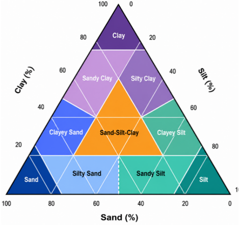
Sediment samples were collected and classified into two primary groups: bed load and suspended load. Bed-load sampling was conducted in accordance with ISO 5667-12:2017, while suspended-load sampling followed the procedures outlined in ISO 5667-17:2000. The collected samples were subsequently analyzed through two main stages: granulometric analysis and gravimetric analysis. Granulometric analysis was performed to determine particle-size distribution, following ISO 1127:2020 (E). The percentages of sand, silt, and clay obtained from the granulometric analysis were subsequently used to classify sediment texture using the soil texture triangle, as illustrated in Figure 3. Gravimetric analysis was used to quantify sediment mass with reference to SNI 06-69398-2004. River discharge measurements were conducted based on SNI 03-2414-1991, which provides guidance for measuring discharge in open channels. Acid digestion was conducted according to SNI 8910:2021 to ensure optimal extraction of heavy metals from the samples. Heavy-metal concentrations in the sediments were then determined using the procedures outlined in SNI 06-6992.3-2004 to evaluate the level of heavy-metal contamination in sediment media.
2.4 Sediment transport calculation
Sediment transport analysis in this study focused on both suspended load and bed load using established empirical formulations [20, 21]. The suspended sediment transport rate was calculated using Eq. (1), which incorporates key hydraulic and sediment parameters, including flow velocity, sediment density, median grain size, and bed shear stress. This formulation reflects the balance between hydrodynamic forces that promote sediment movement and gravitational forces that resist particle suspension.
$q_{s w}=0.05 \times \gamma_s \times v^2 \times\left[\frac{D_{50}}{g\left(\frac{\gamma_s}{y}-1\right)}\right]^{\frac{1}{2}} \times\left[\frac{\tau_0}{\left(\gamma_s-y\right) D_{50}}\right]^{\frac{3}{2}}$ (1)
In this equation, $q_{s w}$ represents the suspended sediment transport rate (ton/day), which is controlled primarily by flow velocity ($v$), sediment density ($\gamma_s$), and median diameter of sediment particles $\left(D_{50}\right)$. The parameter $\gamma$ denotes water density, while $g$ represents gravitational acceleration. Bed shear stress $\left(\tau_0\right)$, which governs sediment entrainment, was calculated using Eq. (2):
$\tau_0=\gamma \times h \times S$ (2)
Here, bed shear stress $\left(\tau_0\right)$ is influenced by water density $(\gamma)$, flow depth $(h)$, and channel slope $(S)$, indicating that deeper flows and steeper gradients enhance sediment mobilization.
Bed-load transport was estimated using Eq. (3), which relates sediment movement along the riverbed to discharge and channel characteristics:
$q_b=\left(39.5 \times Q^{\frac{2}{3}} \times S \times 9.95 \times d\right)^{\frac{3}{2}}$ (3)
In this formulation, $q_b$ denotes the bed-load transport rate (ton/day), which is primarily governed by river discharge (Q), channel slope (S), and representative sediment grain size (d). Higher discharge increases the capacity of the flow to transport sediment along the bed.
The empirical formulas used in this study were selected because they are widely applied to lowland river systems due to their simplicity and minimal data requirements. However, these formulations were originally developed for non-tidal, unidirectional flow conditions. Therefore, their application in estuarine environments, where tidal influences may affect flow direction and velocity, requires careful interpretation. The results presented in this study should therefore be regarded as estimates rather than absolute measured values because they were not verified against direct field measurements of sediment transport.
River discharge measurements were conducted to support sediment transport calculations by determining flow velocity and cross-sectional characteristics during each sampling event. Flow velocity was measured using a flow meter, while discharge was calculated as the product of flow velocity and wetted cross-sectional area, following SNI 03-2414-1991 [22]. The wetted cross-sectional area was obtained by dividing the river into multiple segments to account for spatial variability in depth and width, and by summing the section areas of all segments.
Flow velocity at each vertical was determined using standard point-measurement techniques depending on flow depth, ensuring a representative velocity distribution across the cross-section. This segmented approach allows for a more accurate estimation of discharge by capturing variations in flow conditions within the river channel. Overall, the integration of field measurements and empirical formulations provides a reliable basis for evaluating sediment transport dynamics under natural flow conditions.
2.5 Heavy metal analysis
Heavy-metal analysis in this study was conducted using a combination of SNI standards and the EPA 2002 method. The procedure began with wet digestion using an acid mixture to extract metals from sediment samples. Approximately 2-5 g of a representative sample was placed in a digestion vessel, followed by the addition of 3 mL nitric acid (HNO₃, 65%) and 9 mL hydrochloric acid (HCl, 37%). The mixture was then heated at 120 ℃ to ensure complete decomposition of the sediment matrix and release bound metals into solution. After cooling, the digested sample was filtered using 2.5 μm filter paper to remove residual particulates. The filtrate was subsequently transferred into a 50 mL volumetric flask and diluted with deionized water to achieve a consistent final volume.
Pb concentrations in the samples were determined using Atomic Absorption Spectrophotometry (AAS) with a Buck Scientific 210 VGP instrument (USA). Background correction and matrix modification were applied to improve analytical accuracy. A blank solution containing the same acid composition as the digested samples, namely HCl and HNO₃ diluted to 50 mL, was used to stabilize the baseline. Absorbance measurements were performed at wavelengths of 283.3 nm and 217 nm, with final calibration conducted at 217 nm. To prevent cross-contamination, the aspirator was cleaned between sample measurements. A calibration curve was established using standard solutions, ensuring a correlation coefficient greater than 0.995 to maintain analytical reliability.
Quality assurance and quality control (QA/QC) procedures were applied to ensure analytical reliability. The method detection limit (MDL) and method quantification limit (MQL) for Pb were determined at 0.05 mg/kg and 0.15 mg/kg, respectively. Certified reference material (CRM), namely NIST SRM 2702 Marine Sediment, was analyzed with each batch to verify accuracy, with recoveries ranging from 92% to 107%. All samples were analyzed in duplicate, and the relative standard deviation (RSD) was maintained below 5%. Blank solutions and calibration standards were analyzed every 10 samples to correct for instrument drift. Iron (Fe) was measured independently for each sediment sample using the same AAS method to enable Enrichment Factor (EF) calculations.
The level of sediment contamination was evaluated using the Igeo, which assesses the degree of heavy-metal accumulation relative to background concentrations [23]. In this study, a background value of 0.4 mg/kg was used as the reference [24]. The Igeovalue was calculated using Eq. (4):
$I_{g e o}=\log _2\left[\frac{C_x}{1.5 C_h}\right]$ (4)
In this equation, $I_{g e o}$ represents the Geoaccumulation Index, which indicates the level of sediment contamination. Cx refers to the measured concentration of heavy metals in sediment (mg/kg), whileCb denotes the natural background concentration (mg/kg). The constant factor of 1.5 is introduced to account for natural variations in background values due to lithogenic effects. Based on the calculated Igeo values, contamination levels are classified into categories ranging from uncontaminated to extremely contaminated.
The level of sediment contamination at each sampling location was evaluated using the Igeo, with classifications based on the criteria presented in Table 1 [25, 26].
Table 1. Classification of Geoaccumulation Index (Igeo) values [27]
|
Igeo Value |
Classification |
|
Igeo ≥ 5 |
Extremely contaminated |
|
4 ≤ Igeo< 5 |
Heavily to extremely contaminated |
|
3 ≤ Igeo< 4 |
Heavily contaminated |
|
2 ≤ Igeo< 3 |
Moderately to heavily contaminated |
|
1 ≤ Igeo< 2 |
Moderately contaminated |
|
0 ≤ Igeo < 1 |
Uncontaminated to moderately contaminated |
|
<0 |
Uncontaminated |
Anthropogenic contributions to heavy-metal concentrations in sediments were further assessed using the EF [27]. EF quantifies the degree of metal enrichment relative to natural background levels by normalizing the concentration of the target element against a conservative reference element. In this study, iron (Fe) was used as the reference element, with a measured concentration of 26.308 mg/kg and a background value of 56.3 mg/kg. EF was calculated using Eq. (5) [28]:
$E F=\frac{\left(\frac{C_i}{C_{\text {ref }}}\right) \text { sample }}{\left(\frac{B_i}{B_{\text {ref }}}\right) \text { backgkround }}$ (5)
In this equation, EF represents the Enrichment Factor, indicating the extent of anthropogenic influence. $C_i$ refers to the concentration of the target metal in the sample, while $C_{\text {ref }}$ denotes the concentration of the reference element (Fe) in the sample. Similarly, $B_i$ and $B_{\text {ref }}$ represent the background concentrations of the target metal and the reference element, respectively.
EF values were classified into seven categories, as summarized in Table 2.
Table 2. Classification of Enrichment Factor (EF) value [29]
|
EF Value |
Classification |
|
EF ≤ 1 |
No enrichment |
|
1 < EF ≤ 3 |
Minor enrichment |
|
3 < EF ≤ 5 |
Moderate enrichment |
|
5 < EF ≤ 10 |
Moderately severe enrichment |
|
10 < EF ≤ 25 |
Severe enrichment |
|
25 < EF ≤ 50 |
Very severe enrichment |
|
EF > 50 |
Extremely severe enrichment |
In addition, the Cf was used to evaluate the degree of contamination associated with specific heavy metals [29]. A background value of 20 mg/kg was applied in this analysis. Cf was calculated using Eq. (6):
$C_f=\frac{C_i}{B_i}$ (6)
Here, $C_f$ represents the Contamination Factor, which reflects the level of contamination relative to background conditions. $C_i$ denotes the measured concentration of the heavy metal in sediment (mg/kg), while $B_i$ corresponds to its background concentration (mg/kg).
3.1 Sediment characterization
The study area at the Banjir Kanal Timur estuary is located adjacent to densely populated residential areas, fish auction facilities, and small-scale food businesses. In comparison, the Lamper River, which functions as a tributary, is characterized by high residential density and the direct discharge of domestic wastewater into the river system.
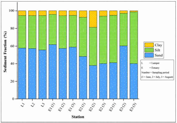
Figure 4 shows that sediment composition varied among the sampling stations and periods. Overall, sand was the dominant sediment fraction at most stations, ranging from 38.51% to 61.20%, while silt ranged from 31.29% to approximately 59.50% and clay ranged from 0.76% to 20.21%. The highest silt content was observed at E3 in August, exceeding the previously reported maximum value of 41.28%. Temporal variations were evident at E2 and E3, where several sampling periods showed an increase in silt content accompanied by a decrease in the sand fraction. The predominance of sand at most stations suggests that the local hydrodynamic conditions were sufficient to transport and deposit relatively coarse sediment particles. In contrast, the higher silt proportions observed at several E2 and E3 samples may indicate lower-energy conditions that facilitated the deposition of finer particles. Clay was the least abundant fraction at nearly all stations, with the highest clay content recorded at E2 in July (20.21%). Potential uncertainty associated with the separation of fine particles during sieving and recovery should be considered when interpreting variations in the clay fraction. Overall, sediment composition exhibited both spatial and temporal variability over the three-month sampling period. Sand was consistently the dominant fraction at stations E1 and, in most sampling periods, at L1–L3, whereas E2 and E3 showed a progressive reduction in sand content accompanied by an increase in silt, indicating a shift toward finer sediment deposition.
Table 3. Bed-load sediment transport from June to August 2024
|
No. |
Month |
Station |
Latitude |
Longitude |
River Width (m) |
Discharge (m3/s) |
D50 (mm) |
qb (ton/day) |
|
1 |
June |
Estuary 1 |
6°57'6.81"S |
110°26'25.48"E |
49.7 |
1.471 |
0.058 |
5.83 × 10⁻⁶ |
|
2 |
June |
Estuary 2 |
6°57'6.63"S |
110°26'25.06"E |
49.7 |
1.471 |
0.062 |
6.45 × 10⁻⁶ |
|
3 |
June |
Estuary 3 |
6°57'6.44"S |
110°26'24.60"E |
49.7 |
1.471 |
0.053 |
5.17 × 10⁻⁶ |
|
4 |
June |
Lamper River |
7°00'6.48"S |
110°26'39.20"E |
12.02 |
0.482 |
0.057 |
1.85 × 10⁻⁶ |
|
5 |
July |
Estuary 1 |
6°57'6.81"S |
110°26'25.48"E |
49.21 |
1.180 |
0.055 |
4.36 × 10⁻⁶ |
|
6 |
July |
Estuary 2 |
6°57'6.63"S |
110°26'25.06"E |
49.21 |
1.180 |
0.051 |
3.81 × 10⁻⁶ |
|
7 |
July |
Estuary 3 |
6°57'6.44"S |
110°26'24.60"E |
49.21 |
1.180 |
0.074 |
6.78 × 10⁻⁶ |
|
8 |
July |
Lamper River |
7°00'6.48"S |
110°26'39.20"E |
11.9 |
0.487 |
0.055 |
1.79 × 10⁻⁶ |
|
9 |
August |
Estuary 1 |
6°57'6.81"S |
110°26'25.48"E |
49.88 |
0.826 |
0.054 |
2.91 × 10⁻⁶ |
|
10 |
August |
Estuary 2 |
6°57'6.63"S |
110°26'25.06"E |
49.88 |
0.826 |
0.051 |
2.69 × 10⁻⁶ |
|
11 |
August |
Estuary 3 |
6°57'6.44"S |
110°26'24.60"E |
49.88 |
0.826 |
0.052 |
2.81 × 10⁻⁶ |
|
12 |
August |
Lamper River |
7°00'6.48"S |
110°26'39.20"E |
11.5 |
0.432 |
0.052 |
1.44 × 10⁻⁶ |
The absence or low proportion of clay in samples from stations E2 and E3 was likely influenced by methodological limitations during the sieving process. The smallest mesh size used in this study (0.063 mm) may not have effectively retained finer clay particles, allowing them to pass through undetected. According to the Wentworth classification, clay particles are defined as having diameters smaller than 0.063 mm, which explains their potential loss during analysis.
Temporal variations in sediment composition reflect dynamic river conditions and are essential for understanding sediment transport processes and their ecological implications. Based on the Shepard triangular classification, sediments from the Lamper River and Estuary 1 were predominantly classified as sand or sandy loam, indicating a high sand content with relatively low proportions of silt and clay. Minor variations in silt and clay fractions were likely influenced by localized changes in flow conditions or sediment sources. Sediment particle-size analysis was conducted sequentially, with coarse fractions separated using a series of sieves of varying mesh sizes. Dried samples were processed using a sieve shaker, allowing finer particles to accumulate in the lower sieves. The finer fractions, including silt and clay, were further analyzed using the pipette method, with sampling time determined based on Stokes’ law, which accounts for particle settling velocity as a function of size and density [30, 31].
3.2 Sediment transport
River discharge measurements were conducted at upstream locations before the estuarine zone to minimize the influence of tidal fluctuations and turbulence commonly present in estuarine environments [31]. Consistent discharge values were assumed across the estuarine sampling points based on the horizontal alignment of the stations, the absence of additional inflows or tributaries between locations, and the relatively uniform river morphology characterized by a gentle slope. This approach is consistent with previous studies that use representative discharge measurements for spatial analysis of sediment dynamics [32, 33]. Channel slope was estimated using elevation data derived from satellite imagery, while flow length was measured using Google Earth Pro. The elevation characteristics of the study reach and the identified tidal type are summarized in Table 4, providing the basis for the hydraulic assumptions adopted in this study. The relatively low flow velocity and gentle river gradient supported the assumption of a constant slope along the study reach. A slope value of 0.011 (1.1%) in the Banjir Kanal Timur River indicates a mild to moderate gradient typical of transitional zones between upstream and coastal areas. This condition facilitates bed-load transport while maintaining relatively stable flow conditions.
In June, bed-load transport calculations based on a modified Meyer-Peter Müller empirical formulation revealed spatial variability across sampling locations. The highest bed-load transport occurred at Estuary 2 (6.45 × 10⁻⁶ ton/day), followed by Estuary 1, while Estuary 3 exhibited slightly lower values despite similar hydrodynamic conditions. The Lamper station consistently showed the lowest transport rate, which can be attributed to its distinct morphological characteristics, including a narrower channel width (12.02 m) and lower discharge (0.482 m³/s), compared with the estuarine stations, which had wider channels of approximately 49.7 m and higher discharge of 1.471 m³/s. These findings highlight the influence of channel geometry and flow conditions on sediment transport capacity.
In July, monitoring results demonstrated notable spatial variation among observation stations. The highest transport rate was recorded at Estuary 3, which is located downstream near artificial infrastructure. Although Estuaries 1 and 2 exhibited similar channel widths (49.21 m) and discharge values, their transport rates differed, indicating the strong influence of local conditions. Estuary 1 exhibited lower transport rates, which may be associated with local hydraulic conditions and the presence of riparian vegetation that increases flow resistance and promotes sediment stabilization. Estuary 2, located in the deepest and central section of the channel, showed relatively stable hydraulic conditions with limited bed-load movement. In contrast, Estuary 3 functioned as an active deposition zone influenced by nearby infrastructure, resulting in higher transport rates due to sediment accumulation. The Lamper station consistently showed the lowest transport rates, reinforcing the strong relationship between sediment transport and local hydrodynamic conditions.
During August, lower flow conditions associated with the dry season reduced the river’s sediment transport capacity. As shown in Table 3, Estuary 1 recorded the highest bed-load transport rate (2.91 × 10⁻⁶ ton/day), followed by Estuary 3 (2.81 × 10⁻⁶ ton/day) and Estuary 2 (2.69 × 10⁻⁶ ton/day), while the Lamper River exhibited the lowest rate (1.44 × 10⁻⁶ ton/day). These variations were associated with differences in discharge, river width, and median diameter of sediment particles (D50) among the sampling stations. The TSS concentration, water depth, and flow velocity obtained from field measurements were used as supporting parameters to characterize the hydrological and sediment conditions at each station.
For bed-load transport, the highest transport rate varied among the sampling stations and months. Estuary 2 exhibited the highest rate in June, reaching 6.45 × 10⁻⁶ ton/day, while Estuary 3 recorded the highest rate in July at 6.78 × 10⁻⁶ ton/day. In August, Estuary 1 showed the highest bed-load transport rate at 2.91 × 10⁻⁶ ton/day. In contrast, the Lamper River consistently exhibited the lowest bed-load transport rates, ranging from 1.44 × 10⁻⁶ to 1.85 × 10⁻⁶ ton/day. These values were calculated from the discharge, river width, and D50 presented in Table 3.
Variations in sediment transport across locations indicate that water depth and TSS concentration are key controlling factors in suspended sediment dynamics. These findings are consistent with previous studies [34], which highlight the influence of discharge, initial sediment concentration, water depth, and flow characteristics on sediment transport processes. Sediment accumulation in estuarine areas can alter channel morphology, reduce water depth, and negatively affect aquatic ecosystems through habitat degradation and disruption of natural flow patterns. Although flow velocity varied among stations, its influence appeared less dominant than TSS concentration in determining transport capacity.
Table 4. Tidal type and elevation data
|
Date |
HHWL (cm) |
MHWL (cm) |
MSL (cm) |
MLWL (cm) |
LLWL (cm) |
Tidal Type |
|
June 24 |
228.37 |
101.84 |
87.29 |
72.75 |
21.23 |
Diurnal |
|
July 24 |
202.69 |
91.84 |
79.38 |
66.92 |
17.26 |
Diurnal |
|
August 24 |
265.60 |
80.59 |
68.27 |
55.94 |
16.28 |
Diurnal |
To support the interpretation of sediment transport dynamics, tidal data from June to August were obtained from BMKG Semarang and IOC Sea Level Monitoring (Table 4). Hourly observations over a 30-day period were analyzed using the Admiralty method to determine tidal range and mean sea level. The results indicate an average sea level of 78.31 cm, with a diurnal tidal pattern characterized by one high tide and one low tide per day. These findings are consistent with previous studies [35, 36], confirming the diurnal tidal regime in Semarang waters. Data collection was conducted during low-tide conditions to minimize tidal interference with sediment transport measurements. The incorporation of tidal information enhances the interpretation of hydrodynamic conditions while supporting the reliability of sediment transport estimates, as indicated in previous research [37, 38].
3.3 Heavy metal content in sediment
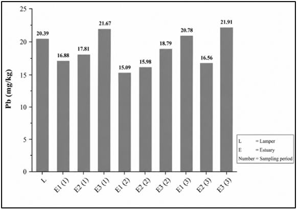
The concentration of heavy metals in sediment samples was determined using Flame AAS. The Pb analysis results presented in Figure 5 show that concentrations ranged from 15.09 to 21.91 mg/kg, indicating the presence of lead contamination in both the Banjir Kanal Timur estuarine system and the Lamper River. Spatial and temporal variations in Pb concentration were observed across sampling locations. As summarized in Table 5, the highest Pb concentration was recorded at Estuary 3 in August (21.91 mg/kg), suggesting that this area received the greatest pollutant input compared with other locations. In contrast, the lowest concentration was observed at Estuary 1 in July (15.09 mg/kg).
Based on the Canadian Sediment Quality Guidelines, all measured Pb concentrations were below the Threshold Effect Level (TEL), indicating a relatively low probability of immediate biological effects. However, these guidelines, although widely applied in both freshwater and marine environments, may have limitations when applied to transitional systems because of differences in natural background conditions [39, 40]. Therefore, for brackish environments such as estuaries, additional indices are required to better capture anthropogenic influences on sediment quality. In this study, the Canadian Freshwater Sediment Quality Guidelines were applied to the Lamper River, while the Canadian Marine Sediment Quality Guidelines were used for estuarine locations because of the absence of specific criteria for brackish systems.
Table 5. Heavy-metal (Pb) test results in sediment
|
No. |
Location |
Result (mg/kg) |
Standard |
|
1 |
Lamper River |
20.39 |
35* |
|
2 |
Estuary 1(1) |
16.88 |
|
|
3 |
Estuary 2(1) |
17.81 |
|
|
4 |
Estuary 3(1) |
21.67 |
|
|
5 |
Estuary 1(2) |
15.09 |
|
|
6 |
Estuary 2(2) |
15.98 |
30.2** |
|
7 |
Estuary 3(2) |
18.79 |
|
|
8 |
Estuary 1(3) |
20.78 |
|
|
9 |
Estuary 2(3) |
16.56 |
|
|
10 |
Estuary 3(3) |
21.91 |
|
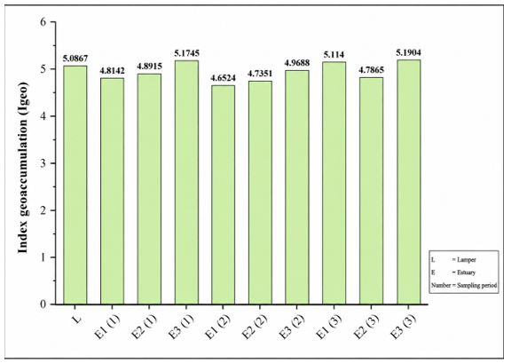
The Igeo values presented in Figure 6 ranged from 4.65 to 5.19. According to the standard classification, these values fall within the “heavily to extremely contaminated” category, indicating substantial Pb accumulation in sediments. The average Igeo value of 4.942 confirms substantial Pb accumulation. However, samples with Igeo values ≥5, such as several samples from E3, fall into the “extremely contaminated” category, while values between 4 and 5 are classified as “heavily to extremely contaminated.” The elevated Igeo values are likely associated with continuous anthropogenic inputs, including industrial discharges and domestic waste, as well as hydrological processes such as flooding that enhance pollutant transport and deposition. The average Igeo value of 4.942 further confirms that the study area is characterized by high contamination levels, which may contribute to long-term ecological degradation and deterioration of aquatic environmental quality.
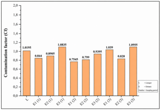
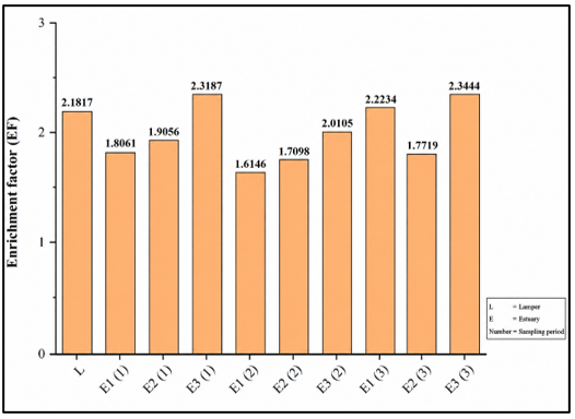
Further assessment using the Cf and EF, as shown in Figure 7 and Figure 8, provides additional insight into contamination sources and intensity. Cf values ranged from 0.755 to 1.096, indicating low to moderate contamination levels, with values greater than one reflecting moderate contamination. Approximately four out of ten samples exhibited Cf values exceeding one, suggesting that nearly half of the study area experienced moderate Pb contamination. However, the overall average Cf value of 0.93 indicates that the general contamination level remains within the low to moderate range. EF values ranged from 1.61 to 2.34, indicating minor enrichment and suggesting a relatively limited contribution from anthropogenic sources. Although some locations exhibited slightly higher EF values, the overall results imply that Pb contamination is influenced by human activities, likely related to surrounding land-use patterns. Notably, Sample 10 from Estuary 3 showed the highest Cf and EF values, indicating localized contamination. Overall, EF results suggest that although anthropogenic inputs are present, their spatial extent across the study area remains relatively limited.
A comparison of Pb concentrations with other locations in the Semarang coastal region (see Table 6) shows that Pb levels in the Lamper River and estuarine stations (E1–E3) were generally higher than those reported in areas such as the Trimulyo Channel, Mangunharjo Channel, and the eastern coast of Semarang [41, 42]. These values also exceed concentrations observed in the Banjir Kanal Barat estuary [43], although they remain slightly lower than the maximum values reported in previous studies of the Banjir Kanal Timur [44]. All measured concentrations remain below the sediment quality guideline threshold of 35 mg/kg.
4.1 Sediment transport rates
Sediment transport rates exhibited distinct spatial and temporal variations, influenced by a combination of physical and hydraulic factors during the observation period. Key controlling parameters include flow velocity, channel slope, sediment particle-size distribution, channel geometry, and tidal forcing. Flow velocity plays a fundamental role in determining the capacity of a river to transport sediment, particularly coarse materials such as sand. Steeper channel slopes increase gravitational energy, thereby enhancing the capacity of the flow to mobilize and transport sediment particles [45, 46]. In addition, D50 serves as an indicator of sediment stability, with coarser particles tending to resist movement and finer particles being more easily entrained and transported in suspension [45]. The interaction among these factors governs sediment transport dynamics across different locations.
Spatial variations were evident among the observation stations. Station E3 consistently exhibited relatively higher bed-load transport rates, which may be associated with nearby concrete structures that potentially induce local flow turbulence and promote sediment resuspension [47, 48]. In contrast, Estuary 1 showed relatively low sediment mobility, which may be influenced by local hydraulic conditions and dense riparian vegetation that enhances sediment retention. Vegetation along riverbanks likely contributes to flow resistance, stabilizes the banks, and reduces flow velocity near the margins, thereby enhancing sediment deposition [49]. However, field measurements of bed roughness and near-bank velocity were not conducted; therefore, these explanations should be considered qualitative inferences. This finding is consistent with previous studies [45], which highlight the significant role of riparian vegetation in regulating sediment flux and stabilizing fluvial systems.
Tidal dynamics further increase the complexity of sediment transport processes in estuarine environments. The study area experiences a diurnal tidal regime, resulting in periodic changes in flow direction and velocity. During flood-tide conditions, reduced flow velocity promotes sediment deposition, whereas during ebb flow, increased flow velocity facilitates downstream sediment transport [50]. This pattern was particularly evident at observation stations 2 and 3. In contrast, the Lamper station, located outside the tidal influence zone, exhibited relatively stable and lower sediment transport rates due to unidirectional flow conditions.
These findings are consistent with previous studies conducted in urban river systems [51], which demonstrate that anthropogenic modifications, such as impermeable surfaces and engineered structures, significantly influence sediment transport processes. Seasonal variability also plays an important role, as highlighted by Patriadi et al. [52], who reported that sediment transport is affected by changes in hydrological conditions and geomorphological characteristics, including slope and vegetation distribution. In this study, dry-season conditions likely enhanced the relative influence of channel morphology and sediment sources, resulting in observable variations in sediment transport across the study area.
4.2 Heavy metal concentration
The concentration of heavy metals in sediment samples in this study is represented by lead (Pb) levels. Based on Table 7, Pb concentrations measured in the Banjir Kanal Timur River and the Lamper River were generally higher than those reported for several other locations. Although these concentrations remain below the TEL, further evaluation using the Igeo, EF, and Cf indicates that anthropogenic activities continue to influence sediment quality. The highest Pb concentration was recorded at Estuary 3 in August, suggesting localized pollutant accumulation. This elevated concentration may be associated with increased land-based activities during the dry season, when reduced river discharge limits the capacity of the water body to dilute contaminants, thereby promoting pollutant accumulation over time.
Sediment characteristics also play a significant role in controlling Pb distribution. Fine-grained particles, particularly silt and clay, have a greater capacity to adsorb heavy metals, resulting in higher Pb concentrations under conditions of elevated TSS [53]. In addition, tidal currents influence the transport and redistribution of suspended particles, thereby affecting Pb distribution patterns within the estuarine system [54]. Local infrastructure, including drainage networks and embankments, further contributes to pollutant dynamics by altering runoff pathways and facilitating the mixing of point and non-point pollution sources.
A notable discrepancy was observed between high $I_{g e o}$ values (4.65-5.19) and moderate $C_f$ values (0.755-1.096). This discrepancy is primarily attributable to the different background values applied. $I_{\text {geo }}$ uses a conservative local baseline background of $0.4 \, \mathrm{mg} / \mathrm{kg}$ [24, 55], employs a logarithmic scale, and incorporates a correction factor of 1.5 to account for natural lithogenic variations, thereby yielding elevated values. In contrast, $C_f$ is calculated as a simple ratio against the global average baseline of $20 \, \mathrm{mg} / \mathrm{kg}$ reported by Wedepohl [56], producing more conservative estimates. Consequently, $I_{\text {geo}}$ indicates "heavily to extremely contaminated" conditions, whereas $C_f$ suggests only low to moderate contamination.
Table 6. Comparison of Pb concentrations from the Semarang coastal area and surrounding locations
|
No. |
Location |
Pb Concentration (mg/kg) |
Unit |
Reference |
|
1 |
Banjir Kanal Timur |
15.09–21.91 |
mg/kg |
This study |
|
2 |
Lamper River |
17.50–20.39 |
mg/kg |
This study |
|
3 |
Banjir Kanal Timur |
14.30–31.35 |
ppm |
[44] |
|
4 |
Tanjung Mas Harbor |
0.67–0.73 |
mg/kg |
[57] |
|
5 |
Mangunharjo Waterway |
0.220–0.280 |
mg/kg |
[57] |
|
6 |
Banjir Kanal Barat Estuary |
4.14–13.93 |
ppm |
[43] |
|
7 |
Trimulyo Waterway |
0.030–5.96 |
mg/kg |
[41] |
|
8 |
Mangunharjo Waterway |
0.030–3.69 |
mg/kg |
[41] |
|
9 |
Semarang East Coast |
0.030–6.23 |
mg/kg |
[42] |
The primary sources of Pb contamination in the study area are associated with industrial activities and urban development, particularly automotive-related operations, informal metal processing, and small-scale manufacturing. Additional contributions may arise from vehicle brake wear, tire residues, and the recycling of batteries and electronic waste. Previous studies have shown that metal pollution in similar environments often originates from multiple sources, including natural, traffic-related, industrial, and mixed contributions [58]. Isotopic analyses further indicate that Pb contamination may be dominated by natural sources and coal combustion, with a smaller contribution from traffic emissions [59].
A comparison of Pb concentrations with other locations in the Semarang coastal region (see Table 7) shows that Pb levels in the Lamper River and estuarine stations (E1–E3) were generally higher than those reported in areas such as the Trimulyo Channel, Mangunharjo Channel, and the eastern coast of Semarang [56, 57]. These values also exceed concentrations observed in the Banjir Kanal Barat estuary [55], although they remain slightly lower than the maximum values reported in previous studies of the Banjir Kanal Timur [53]. Furthermore, Pb concentrations in sediments were significantly higher than those reported in biota, such as Perna viridis from Tanjung Mas Harbor and surrounding waterways [54]. Despite these differences, all measured concentrations remain below the sediment quality guideline threshold of 35 mg/kg.
The apparent discrepancy between high Igeo values (4.652–5.190) and relatively low to moderate Cf values (0.755–1.096) can be attributed to differences in calculation approaches and reference baselines. The Igeo index employs a logarithmic scale and incorporates a correction factor, typically 1.5, to account for natural geochemical variability, which tends to produce higher values. In addition, the choice of background concentration significantly influences the results. This study uses a relatively low baseline value of 0.4 mg/kg [58], compared with the global average of 20 mg/kg [59], resulting in elevated Igeo values. In contrast, Cf is calculated as a simple ratio between measured and background concentrations, producing more conservative estimates. Consequently, Igeo indicates “heavily to extremely contaminated” conditions, whereas Cf suggests only moderate contamination.
The EF values obtained in this study (1.61–2.34) indicate minor to moderate enrichment, suggesting a measurable but not dominant contribution from anthropogenic sources. Because EF values are independent of absolute background values, they confirm that anthropogenic inputs are present but relatively limited. The highest EF value was observed at Estuary 3, which is located near industrial and automotive-related activities, supporting the interpretation of localized human influence. In contrast, lower EF values at Estuary 1 may reflect the mitigating effect of riparian vegetation and reduced pollutant input from upstream areas. Therefore, the combined interpretation of all three indices suggests that the study area is best characterized as experiencing low to moderate Pb contamination with localized anthropogenic pressure, rather than the “extremely contaminated” category implied by Igeo alone.
Potential sources of Pb contamination in the study area may be associated with surrounding land-use activities, including automotive workshops, small-scale metal industries, and domestic runoff. However, because no source-apportionment analysis, such as isotope analysis, detailed land-use inventory, or discharge survey, was conducted in this study, these attributions should be considered possible sources based on typical urban pollution patterns rather than definitive conclusions.
Overall, Pb concentrations in the Banjir Kanal Timur and Lamper River are consistent with other reports from Java, although they are lower than concentrations reported in heavily polluted sites such as Tirang Beach (49.16 mg/kg) and the Citarum River, where concentrations reach up to 80 mg/kg. Conversely, significantly lower Pb levels have been reported in less impacted areas such as the Madura Strait (0.12–2.01 mg/kg), reflecting minimal anthropogenic influence [58]. Based on the combined interpretation of Cf, Igeo, and EF values, the study area can be classified as experiencing moderate pollution with notable anthropogenic pressure.
Urban water bodies in Semarang tend to exhibit elevated Pb concentrations due to intensive land use and urban runoff, consistent with patterns observed in other Indonesian urban systems. In contrast, offshore environments typically show lower Pb concentrations due to dilution by seawater, sediment deposition in low-energy zones, and geochemical processes such as oxidation and complexation [60]. Tidal processes also contribute to the redistribution of metals across wider areas, leading to localized decreases in concentration, as observed in Jakarta Bay [61]. A similar mechanism is likely present in the Banjir Kanal Timur estuary, where sediments act as temporary sinks for heavy metals before their eventual transport to marine environments.
Spatial and temporal variations in sediment transport within the Banjir Kanal Timur River are primarily controlled by river discharge, sediment grain size, channel morphology, and tidal dynamics. The highest bed-load transport was observed at Estuary 3 in July (6.78 × 10⁻⁶ tons/day), likely influenced by the presence of concrete infrastructure that may enhance flow turbulence and sediment remobilization. In contrast, the highest suspended-load transport occurred at Estuary 2 (3.81 × 10⁻² tons/day), which was associated with greater water depth and sediment availability. The Lamper River consistently exhibited the lowest transport rates due to its narrower channel and lower discharge. Variations in suspended sediment transport across locations and time further demonstrate the complex interaction between hydrodynamic conditions and sediment characteristics.
Pb concentrations in sediment samples ranged from 15.09 to 21.91 mg/kg across all sampling locations. Although these values remain below the Canadian TEL (35 mg/kg), the Igeoindicates conditions ranging from heavily to extremely contaminated (4.65–5.19), largely influenced by the use of a conservative background value (0.4 mg/kg). The Cf, ranging from 0.755 to 1.096, suggests low to moderate contamination levels, while EF values between 1.61 and 2.34 indicate minor anthropogenic enrichment, particularly in estuarine areas. Considering the combined indices, the study area is best classified as experiencing moderate Pb contamination with localized anthropogenic pressure.
Overall, the findings suggest that Pb contamination in the study area is primarily associated with surrounding land-use activities, including potential contributions from automotive services, small-scale metal industries, and domestic runoff. Compared with other regions in Semarang and across Indonesia, the Banjir Kanal Timur estuary system can be categorized as moderately affected by urban-derived heavy-metal pollution.
This work was supported by Universitas Diponegoro through the International Publication Research Scheme (RPI), under Assignment Letter No. 222-536/UN7.D2/PP/IV/2025.
[1] APPAMSI. (2019). The benefits of water resources in daily life. https://appamsi.co.id/manfaat-sumber-daya-air-dalam-kehidupan-sehari-hari/.
[2] Swartz, J., Standring, P., Goff, J.A., Gulick, S., Lowery, C.M. (2022). Coastal river response to transgression: A new look at the Trinity incised valley using multi-resolution seismic imaging. EarthArXiv, 1-33. https://doi.org/10.31223/X5P044
[3] Sudarno, Wibowo, M.A., Andarini, P., Puspita, A.S., Humaira, N.G., Putri, N.N.A. (2024). Mitigating the drinking water crisis in developing regions-A comprehensive evaluation of disinfection technologies. Ecological Engineering & Environmental Technology, 25: 85. https://doi.org/10.12912/27197050/184377
[4] Pambudi, N.A.R., Handoyo, G., Rochaddi, B. (2023). Estimated sedimentation rate in the Silugonggo River Estuary, Pati Regency. Indonesian Journal of Oceanography, 5: 43-56. https://doi.org/10.14710/ijoce.v5i1.15835
[5] Tamansari, A.M.D., Sekitarnya, K.T. (2023). Morphotectonic analysis of the Tamansari area and its surroundings, Tanggamus Regency, Lampung. Journal of Geology Sriwijaya, 2(1): 33-41. https://pdfs.semanticscholar.org/b76e/60efa94a9e42785c3e8b40a6c0bd5d05f6a6.pdf.
[6] Mohanavelu, A., Shrivastava, S., Naganna, S.R. (2022). Streambed pollution: A comprehensive review of its sources, eco-hydro-geo-chemical impacts, assessment, and mitigation strategies. Chemosphere, 300: 134589. https://doi.org/10.1016/j.chemosphere.2022.134589
[7] Sari, D.K., Budihardjo, M.A., Puspita, A.S., Firmansyah, F., Zenith, I.T. (2026). Bibliometric review of ballast water management within the framework of the circular economy. Cleaner Water, 5: 100213. https://doi.org/10.1016/j.clwat.2026.100213
[8] Aggarwal, M., Anbukumar, S., Kumar, T.V. (2025). The relationship between pH, organic matter and heavy metal concentrations in surface sediment of Ganga River, India. Water Environment Research, 97: e70160. https://doi.org/10.1002/wer.70160
[9] Maqsood, A., Łobos-Moysa, E. (2025). Bottom sediments as dynamic arenas for anthropogenic pollutants: Profiling sources, unraveling fate mechanisms, and assessing ecological consequences. International Journal of Molecular Sciences, 26: 10219. https://doi.org/10.3390/ijms262010219
[10] Muskananfola, M.R., Hartoko, A., Latifah, N. (2023). Assessment of heavy metal Cd and Pb concentrations and the ecological risk from seawater, sediments, and Perna viridis in Semarang Bay, Indonesia. Applied Environmental Research, 45(2). https://doi.org/10.35762/AER.2023013
[11] Puspita, A.S., Budihardjo, M.A., Chegenizadeh, A., Nikraz, H., Sania, M.T., Andini, A.M. (2026). Marine debris governance and regional dynamics in Southeast Asia. Cleaner Water, 100231. https://doi.org/10.1016/j.clwat.2026.100231
[12] Le, H.P., Pham, H.N., Le, T.D., et al. (2024). Heavy metals assessment for sustainable management in estuaries of Ba Ria-Vung Tau Province. Viet Nam Journal of Marine Science and Technology, 24(1): 17-32. https://doi.org/10.15625/1859-3097/18976
[13] Ma, Y., Ma, Y., Zhang, W.J., et al. (2024). The spatiotemporal variation and historical evolution of heavy metal pollution in sediments from the Pearl River Estuary, China. Water, 16: 531. https://doi.org/10.3390/w16040531
[14] Wang, F., Hao, R.J. (2020). Environmental pollution in Pearl River Delta, China: Status and potential effects. Journal of Environmental Informatics Letters, 3: 110-123. https://doi.org/10.3808/jeil.202000033
[15] Hastuti, E.D. (2021). Increasing risk of heavy metal contamination in silvofishery ponds. Biotropia, 28: 38-45. https://orcid.org/0000-0002-9923-1110
[16] Wu, W., Wu, P., Yang, F., Sun, D.L., Zhang, D.X., Zhou, Y.K. (2018). Assessment of heavy metal pollution and human health risks in urban soils around an electronics manufacturing facility. Science of the Total Environment, 630: 53-61. https://doi.org/10.1016/j.scitotenv.2018.02.183
[17] Zhao, Y.F., Shi, X.Z., Huang, B., et al. (2007). Spatial distribution of heavy metals in agricultural soils of an industry-based peri-urban area in Wuxi, China. Pedosphere, 17: 44-51. https://doi.org/10.1016/S1002-0160(07)60006-X
[18] Sheng, P., Yu, Y.Z., Zhang, G.H., Huang, J.L., He, L., Ding, J.N. (2016). Bacterial diversity and distribution in seven different estuarine sediments of Poyang Lake, China. Environmental Earth Sciences, 75: 479. https://doi.org/10.1007/s12665-016-5346-6
[19] Shepard, F.P., Moore, D. (1954). Sedimentary environments differentiated by coarse-fraction studies. AAPG Bulletin, 38: 1792-1802. https://doi.org/10.1306/5CEAE031-16BB-11D7-8645000102C1865D
[20] Balouchi, B., Rüther, N., Schwarzwälder, K. (2024). Temporal variation of braided intensity and morphodynamic changes in a regulated braided river using 2D modeling and satellite images. River Research and Applications, 40: 708-724. https://doi.org/10.1002/rra.4268
[21] Le Minor, M., Davy, P., Howarth, J., Lague, D. (2022). Multi grain-size total sediment load model based on the disequilibrium length. Journal of Geophysical Research: Earth Surface, 127: e2021JF006546. https://doi.org/10.1029/2021JF006546
[22] National Standardization Agency. (1991). Methods for Measuring River and Open Channel Discharge. National Standardization Agency. https://dewey.petra.ac.id/view/143980.
[23] Navarrete-Rodríguez, G., Castañeda-Chávez, M.d.R., Lango-Reynoso, F. (2020). Geoacumulation of heavy metals in sediment of the fluvial-lagoon-deltaic system of the Palizada River, Campeche, Mexico. International Journal of Environmental Research and Public Health, 17: 969. https://doi.org/10.3390/ijerph17030969
[24] Nawrot, N., Wojciechowska, E., Mohsin, M., Kuittinen, S., Pappinen, A., Rezania, S. (2021). Trace metal contamination of bottom sediments: A review of assessment measures and geochemical background determination methods. Minerals, 11: 872. https://doi.org/10.3390/min11080872
[25] Tuo, A.D., Traoré, I.B.C., Trokourey, A. (2023). Use of several pollution indices for metal contamination assessment in aquatic ecosystems, a case study, Ebrié Lagoon-Côte d'Ivoire. In Heavy Metals-Recent Advances. IntechOpen. https://doi.org/10.5772/intechopen.110244
[26] Pradit, S., Noppradit, P., Jitkaew, P., et al. (2022). Heavy metal contamination and ecological risk assessment in the sediment cores of the wetlands in Southern Thailand. Journal of Marine Science and Engineering, 10: 1921. https://doi.org/10.3390/jmse10121921
[27] Xie, S.W., Liu, C.S., He, B., et al. (2022). Geochemical fractionation and source identification of Pb and Cd in riparian soils and river sediments from three lower reaches located in the Pearl River Delta. International Journal of Environmental Research and Public Health, 19: 13819. https://doi.org/10.3390/ijerph192113819
[28] Imsilp, K., Sirinupong, P., Yeesin, P., Thong-Asa, W., Tanhan, P. (2025). Potential risks and spatial variation of heavy metals in water and surface sediment of Pattani Bay, Thailand. Toxics, 13: 477. https://doi.org/10.3390/toxics13070477
[29] Rodrigues, B.B., Mizusaki, A.M.P., Menegat, R., de Figueiredo, A.R., Galligan, T.A., Portella, M.B.P. (2021). Contamination of urban watersheds: The case of Arroio Moinho, Porto Alegre, Rio Grande do Sul, Brazil. Anuário do Instituto de Geociências, 44. https://doi.org/10.11137/1982-3908_2021_44_36551
[30] Aquilano, A., Marrocchino, E., Paletta, M.G., Tessari, U., Vaccaro, C. (2023). Geochemical characterization of sediments from the Bibione coastal area (northeast Italy): Details on bulk composition and particle size distribution. Journal of Marine Science and Engineering, 11: 1650. https://doi.org/10.3390/jmse11091650
[31] Hamarashid, R.A., Fiket, Ž., Mohialdeen, I.M. (2022). Environmental impact of Sulaimani steel plant (Kurdistan Region, Iraq) on soil geochemistry. Soil Systems, 6: 86. https://doi.org/10.3390/soilsystems6040086
[32] Ahamad, M.I., Yao, Z.J., Ren, L., et al. (2024). Impact of heavy metals on aquatic life and human health: A case study of River Ravi Pakistan. Frontiers in Marine Science, 11: 1374835. https://doi.org/10.3389/fmars.2024.1374835
[33] Silva, T.A.d.C., Paula Jr, M.d., Silva, W.S., Lacorte, G.A. (2021). Deposition of potentially toxic metals in the soil from surrounding cement plants in a karst area of Southeastern Brazil. Conservation, 1(3): 137-150. https://doi.org/10.3390/conservation1030012
[34] Sucipto, A., Thaha, M.A., Hatta, M.P., Mahmuddin, F. (2025). Sedimentation characteristics and sediment transport in the Palu River Estuary. Civil Engineering Journal, 11(2).
[35] Az Zahro, A., Zahrina, W.N. (2024). Tidal type analysis for determining sea level elevation in Semarang waters using the Admiralty method. Jurnal Hidrografi Indonesia, 6: 7-14. https://doi.org/10.62703/jhi.v6i1.55
[36] Jiang, X.Z., Lu, B., He, Y.H. (2013). Response of the turbidity maximum zone to fluctuations in sediment discharge from river to estuary in the Changjiang Estuary (China). Estuarine, Coastal and Shelf Science, 131: 24-30. https://doi.org/10.1016/j.ecss.2013.07.003
[37] Nugroho, E.O., Pranatan, A.Y., Soekarno, I., et al. (2024). The effect of discharge, sediment transport, tidal and land subsidence in the river flood risk management: Case study of Sayung River. In Journal of Physics: Conference Series, 2916: 012017. https://doi.org/10.1088/1742-6596/2916/1/012017
[38] Gemilang, W.A., Wisha, U.J., Solihuddin, T., Arman, A., Ondara, K. (2020). Sediment accumulation rate in Sayung Coast, Demak, Central Java using unsupported 210Pb isotope. Atom Indonesia, 46: 25-32. https://doi.org/10.17146/aij.2020.935
[39] Chaya, T.M., Schafer, T.B., Osborne, T.Z. (2023). Assessing water quality dynamics in tidally influenced blackwater rivers along a rural-urban gradient. Water, 15: 4154. https://doi.org/10.3390/w15234154
[40] Emeka, C.N., Emeka, V.I., Itam, A., et al. (2026). Physicochemical characteristics of the Great Kwa River (Gulf of Guinea): Controls of tidal dynamics and environmental sustainability in a tropical mesotidal system. https://doi.org/10.21203/rs.3.rs-9595578/v1
[41] Moodie, A.J., Nittrouer, J.A., Ma, H., et al. (2022). Suspended sediment-induced stratification inferred from concentration and velocity profile measurements in the Lower Yellow River, China. Water Resources Research, 58: e2020WR027192. https://doi.org/10.1029/2020WR027192
[42] Ikhsan, C. (2023). The effect of shear stress on armor layer thickness under steady uniform flow. Civil Engineering Journal, 9: 2806-2822. https://doi.org/10.28991/CEJ-2023-09-11-012
[43] Biggs, H.J., Haddadchi, A., Hicks, D.M. (2021). Interactions between aquatic vegetation, hydraulics and fine sediment: A case study in the Halswell River, New Zealand. Hydrological Processes, 35: e14245. https://doi.org/10.1002/hyp.14245
[44] Kumar, P., Sharma, A. (2025). Experimental analysis of vegetation heterogeneity on flow characteristics and bed morphology in partially vegetated channels. Earth Surface Processes and Landforms, 50: e70174. https://doi.org/10.1002/esp.70174
[45] Wang, M., Mi, S., Avital, E., Li, N., Chen, Y., Williams, J. (2023). A study on the influence of submergence ratio on the transport of suspended sediment in a partially vegetated channel flow. Water Resources Research, 59(3): e2022WR032876. https://doi.org/10.1029/2022WR032876
[46] Isma, F., Ismida, Y., Isma, M.F., Sufahani, S.F., Akbar, H. (2023). Effect of stream river and tidal on the suspended sediment concentration of Kuala Langsa Estuary, Aceh, Indonesia. Ilmu Kelautan: Indonesian Journal of Marine Sciences, 28(1): 27-36. https://doi.org/10.14710/ik.ijms.28.1.27-36
[47] Dsikowitzky, L., Van der Wulp, S.A., Ariyani, F., Hesse, K.J., Damar, A., Schwarzbauer, J. (2018). Transport of pollution from the megacity Jakarta into the ocean: Insights from organic pollutant mass fluxes along the Ciliwung River. Estuarine, Coastal and Shelf Science, 215: 219-228. https://doi.org/10.1016/j.ecss.2018.10.017
[48] Patriadi, A., Soemitro, R.A.A., Warnana, D.D. (2024). Seasonal variations in sediment characteristics at the estuary of Bengawan Solo River: A study of river branching and flow velocity influences. In AIP Conference Proceedings, 3110: 020054. https://doi.org/10.1063/5.0205082
[49] Xie, W., Sun, J., Guo, L., et al. (2023). Distinctive sedimentary processes on two contrasting tidal flats of the Yellow River Delta. Frontiers in Marine Science, 10: 1259081. https://doi.org/10.3389/fmars.2023.1259081
[50] Bilal, A., Xie, Q.C., Zhai, Y.Y. (2020). Flow, sediment, and morpho-dynamics of river confluence in tidal and non-tidal environments. Journal of Marine Science and Engineering, 8: 591. https://doi.org/10.3390/jmse8080591
[51] Afifudin, A.F.M., Pramesti, H.N., Irawanto, R., et al. (2025). Spatial distribution and risk assessment of heavy metal contamination in western Madura Strait sediments. Results in Engineering, 26: 105157. https://doi.org/10.1016/j.rineng.2025.105157
[52] Taylor, S.R. (1964). Abundance of chemical elements in the continental crust: A new table. Geochimica et Cosmochimica Acta, 28: 1273-1285. https://doi.org/10.1016/0016-7037(64)90129-2
[53] Putra, M.D.N., Widada, S., Atmodjo, W. (2022). Study of lead (Pb) heavy metal content in bottom sediments in the east flood canal waters of Semarang. Indonesian Journal of Oceanography, 4: 13-21. https://doi.org/10.14710/ijoce.v4i3.13398
[54] Siringoringo, V.T., Pringgenies, D., Ambariyanto, A. (2022). Study of the heavy metal content of mercury (Hg), copper (Cu), and lead (Pb) in Perna viridis in Semarang City. Journal of Marine Research, 11: 539-546. https://doi.org/10.14710/jmr.v11i3.33864
[55] Maslukah, L. (2013). The relationship between the concentrations of heavy metals Pb, Cd, Cu, Zn with organic material and grain size in sediments in the west flood canal estuary, Semarang. Buletin Oseanografi Marina, 2: 55-62. https://ejournal.undip.ac.id/index.php/buloma/article/view/6951.
[56] Mirawati, F., Supriyantini, E., Nuraini, R.A.T. (2016). Content of heavy metal lead (Pb) in water, sediment, and green mussels (Perna viridis) in Trimulyo and Mangunharjo Waters, Semarang. Buletin Oseanografi Marina, 5: 121-126. https://doi.org/10.14710/buloma.v5i2.15731
[57] Testi, E.H., Soenardjo, N., Pramesti, R. (2019). Pb metal in Avicennia marina Forssk, 1844 (Angiosperms: Acanthaceae) in water environment, sediment, on the east coast of Semarang. Journal of Marine Research, 8: 211-217. https://doi.org/10.14710/jmr.v8i2.25212
[58] Chen, X.D., Lu, X.W. (2018). Contamination characteristics and source apportionment of heavy metals in topsoil from an area in Xi'an city, China. Ecotoxicology and Environmental Safety, 151: 153-160. https://doi.org/10.1016/j.ecoenv.2018.01.010
[59] Yu, H., Organ, H., Xu, D., Coffin, R. (2023). Tidal control and mangrove dieback impact on methane emissions from a subtropical mangrove estuary. Limnology and Oceanography, 68: 753-766. https://doi.org/10.1002/lno.12307
[60] Tang, D.B., Luo, S.Y., Deng, S.Y., Huang, R., Chen, B.S., Deng, Z.Y. (2022). Heavy metal pollution status and deposition history of mangrove sediments in Zhanjiang Bay, China. Frontiers in Marine Science, 9: 989584. https://doi.org/10.3389/fmars.2022.989584
Kusuma, A.H., Prartono, T., Atmadipoera, A.S., Arifin, T. (2015). Distribution of dissolved and deposited heavy metals in the waters of Jakarta Bay. Jurnal Teknologi Perikanan dan Kelautan, 6: 41-49. https://doi.org/10.24319/jtpk.6.41-49