Spatial and Seasonal Assessment of Nutrients and E. coli Contamination in Coastal Domestic Wells of Tanah Laut Regency

Groundwater is an essential source of domestic water in many coastal communities, particularly where access to centralized piped water is limited, and households rely on shallow wells for daily needs [1, 2]. Ensuring safe groundwater is directly linked to the achievement of Sustainable Development Goal 6, which emphasizes universal access to safe drinking water, improved sanitation, and reduced water pollution [1]. However, shallow coastal aquifers are highly vulnerable because they are often unconfined, close to the land surface, affected by seawater intrusion, and exposed to pollutant inputs from settlements, sanitation systems, agriculture, and other coastal land-use activities [3-5].

Groundwater quality in coastal areas is influenced not only by salinity, but also by anthropogenic contaminants such as nutrients and fecal microorganisms. Nutrients such as ammonia, nitrate, and phosphate are commonly associated with domestic wastewater, septic tank leakage, livestock waste, fertilizer use, detergents, and other nutrient-rich sources [4, 6]. Nitrate is of particular concern because elevated concentrations in drinking water may pose health risks, especially for vulnerable populations [3, 7]. Ammonia and phosphate can also indicate organic pollution, wastewater infiltration, and nutrient enrichment in shallow groundwater systems [5, 6].

Microbiological contamination is another critical concern for groundwater used as a domestic water source. The presence of Escherichia coli indicates fecal contamination and suggests that pathogens from human or animal waste may have entered the groundwater system [4, 8]. Studies in Indonesia have shown that microbial contamination of shallow groundwater is associated with well type, poor well protection, sanitation conditions, proximity to septic systems, and local hydrogeological factors [9, 10]. In low-lying coastal settlements, shallow water tables and limited separation between wells and sanitation facilities can increase the risk that wastewater-derived nutrients and fecal bacteria migrate into domestic wells [11, 12].

Coastal aquifers require integrated assessment because nutrient enrichment, fecal contamination, seawater intrusion, and land-use pressures may occur simultaneously [5, 13-15]. Previous studies have shown that coastal groundwater contamination can reflect combined influences from domestic sewage, agriculture, aquaculture, and hydrogeochemical processes [14-16]. Therefore, groundwater assessment in coastal areas should not rely on a single parameter, but should consider chemical indicators, microbiological indicators, spatial position, and potential contamination sources together [6, 14, 17].

Geographic information systems, or GIS, provide an effective approach for assessing and visualizing spatial variation in groundwater quality. GIS-based groundwater studies can support the classification of water quality, identification of vulnerable zones, overlay analysis of potential sources, and spatial interpretation of contamination patterns [18-20]. By integrating laboratory measurements with information on well locations, distance from the coastline, and distance from sanitation facilities, GIS-based assessment can help identify areas where groundwater protection and sanitation improvement should be prioritized [18-20].

Tanah Laut Regency, South Kalimantan, contains coastal sub-districts such as Takisung, Panyipatan, Jorong, and Kintap, where shallow groundwater remains important for domestic use and where coastal settlements, sanitation systems, agriculture, and other land-use activities may place pressure on groundwater quality [21, 22]. Despite this vulnerability, spatially explicit information on nutrient contamination and E. coli occurrence in domestic wells in these coastal areas remains limited. This lack of integrated chemical, microbiological, and spatial information constrains local efforts to identify high-risk zones and design targeted groundwater protection strategies [18, 21, 22]. The groundwater-quality classification and scoring criteria used to evaluate nitrate, ammonia, phosphate, and E. coli are presented in Table 1. These criteria were applied consistently to classify the measured water-quality parameters into five quality levels.

This study addresses the following research question: How do nutrient concentrations and E. coli contamination vary spatially in shallow coastal groundwater in Takisung, Panyipatan, Jorong, and Kintap, and how can GIS-based assessment be used to identify groundwater vulnerability zones? The specific contribution of this study is the integration of laboratory measurements of ammonia, nitrate, phosphate, and E. coli with GIS-based spatial analysis of well locations, coastal proximity, and sanitation-related factors. By classifying groundwater quality and mapping contamination patterns, this study provides locally relevant evidence for groundwater protection, sanitation planning, and safer domestic water access in coastal Tanah Laut Regency.

3.1 Spatial distribution of groundwater nutrient concentrations

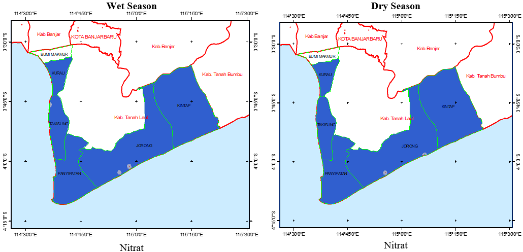
The seasonal nitrate pattern may reflect the combined influence of dilution, leaching, and persistent anthropogenic inputs. Higher rainfall during the wet season may dilute nitrate in shallow groundwater, but it may also promote leaching of residual nitrogen from fertilizers, organic waste, and other surface-derived sources into the aquifer [43]. Conversely, during the dry season, reduced recharge and increased evapotranspiration may contribute to higher nitrate concentrations, while lower rainfall may reduce nitrogen leaching from the soil surface [42]. These opposing processes may explain why nitrate concentrations remained within a comparable range between seasons. However, because rainfall intensity, groundwater level, infiltration rate, redox condition, groundwater flow direction, and pumping intensity were not directly measured, dilution, leaching, and evaporative concentration should be regarded as possible explanations rather than confirmed mechanisms. Similar seasonal patterns have been reported in agricultural groundwater systems, where anthropogenic inputs such as fertilizer, livestock manure, and domestic waste may have a stronger influence than short-term seasonal variability [44].

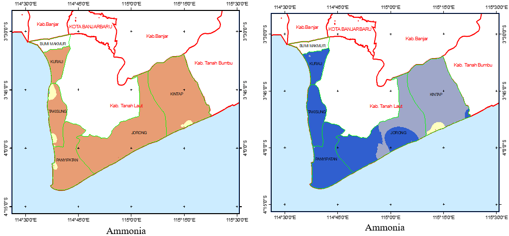
The land-use distribution of the study area is presented in Figure 2. The map shows that residential areas are located near agricultural land and aquaculture areas, providing spatial context for interpreting the observed groundwater-quality patterns. Figure 3 shows a more heterogeneous pattern for ammonia parameters compared to nitrate, with some wells remaining in the good to excellent category (marked in light and dark blue), while others shifted to the moderate to poor category (yellow to orange). This variation indicates that the formation and transformation of ammonia in the Tanah Laut coastal aquifer is highly dependent on local hydrogeological conditions and the intensity of anthropogenic activities, particularly fertilization practices and domestic waste disposal. During the rainy season, the increase in the number of points in the lower quality category reflects the accumulation of ammonia originating from the decomposition of organic matter and nitrogen fertilizers that have not been fully oxidized to nitrate, particularly in shallow aquifers with redox conditions that tend to be reductive. Nitrogen transformation in groundwater is strongly influenced by redox (reduction-oxidation) conditions, thus potentially accumulating ammonia in zones with limited oxygen circulation and low oxidation capacity [45].

Conversely, during the dry season, ammonia quality was observed in a number of wells, as indicated by a shift in the category toward blue. This phenomenon can be attributed to increased ammonia oxidation to nitrate as the groundwater level drops and the aeration zone thickness increases, increasing the opportunity for contact between water and oxygen. However, in several locations hydrogeologically trapped in reductive conditions or subjected to continuous domestic and livestock waste, ammonia levels remained in the moderate to poor category. This condition indicates multiple sources of contamination, originating not solely from agricultural fertilizer residues but also from household waste and livestock activities around the wells [46].

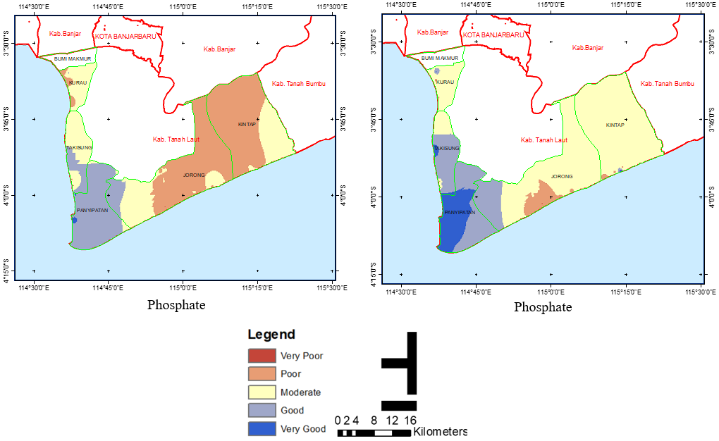
Figure 3 shows significant spatial and temporal variations in phosphate levels between the rainy and dry seasons. During the rainy season, phosphate levels tend to increase in coastal zones with high activity levels, reflected in the dominance of moderate to very poor quality classes (categories 3–1) in several coastal sub-districts. This condition indicates that surface phosphate input from agricultural activities, settlements, and coastal tourism exceeds the natural dilution and filtration capacity of shallow aquifers. This pattern aligns with the findings of various studies in tropical coastal areas, which show that increased rainfall strengthens surface runoff and accelerates phosphate transport from land to shallow groundwater systems [47, 48].

Conversely, during the dry season, the distribution pattern of residual phosphate shifts significantly. Several areas that were in the moderate to poor category during the rainy season gradually improved in quality to good to excellent (categories 4–5), as illustrated by the dominance of light and dark blue colors in several coastal segments. Similar phenomena have been reported in coastal hydrological studies that emphasize the role of seasonal rainfall variability on the dynamics of nutrient concentrations in groundwater, where the dry season tends to produce a pattern of stabilization or decrease in phosphate levels after the peak load during the rainy season [49, 50].

From a hydrogeological perspective, the seasonal variations depicted in the map can be interpreted as a manifestation of the balance between recharge and discharge processes in shallow coastal aquifer systems. During the rainy season, intensive rainwater infiltration increases recharge volume while accelerating the movement of phosphate from the topsoil toward the saturated zone. Consequently, although groundwater volume increases, phosphate concentrations increase, particularly in locations with high nutrient loads. As explained by Foster and Chilton [51] and furthered in various coastal groundwater studies, shallow aquifers in tropical coastal areas are highly susceptible to nutrient contamination due to their relatively shallow depth and proximity to surface pollution sources. During the dry season, decreased rainfall and reduced runoff result in fewer new phosphate inputs, so that phosphate concentrations are largely determined by release mechanisms, lateral flow, and well water pumping, which can help reduce nutrient loads in some locations.

Consistent with the literature, exposure to nitrate and ammonia at concentrations exceeding drinking water quality standards is associated with an increased risk of methemoglobinemia, impaired thyroid function, and the potential formation of carcinogenic N-nitroso compounds in the human body [52, 53]. In the context of the Tanah Laut coastal area, which relies heavily on well water, the presence of a number of wells of moderate to very poor quality directly increases public health vulnerabilities, particularly among children, pregnant women, and the elderly. Furthermore, the accumulation of phosphate and nitrate leaching from aquifers into surface water bodies can accelerate eutrophication, reduce dissolved oxygen levels, and damage coastal ecosystems, ultimately leading to reduced productivity of capture fisheries and aquaculture, which are sources of livelihood for local communities [54].

Normatively, these findings relate to the obligation of local governments and agricultural businesses to implement the precautionary principle in fertilizer use and environmental quality management, as stipulated in various national regulations regarding water resource management and environmental protection. From the perspective of environmental law and Islamic jurisprudence, fertilization practices that lead to well water pollution can be viewed as a violation of the principle of la darar wa la dirar (not causing harm to oneself or others). Therefore, a policy approach is needed that integrates positive legal instruments, administrative oversight, and the internalization of religious values into the ecological behavior of communities and businesses [53, 55].

Based on the identified seasonal contamination patterns, one key strategy that can be developed is the implementation of site-specific nutrient management, which regulates the dosage, timing, and method of fertilizer application to meet plant needs while minimizing nutrient loss to the environment. This practice includes, among other things, avoiding fertilizer application before or during forecasted high rainfall to reduce the risk of leaching and runoff of fertilizer residues into shallow aquifers [55]. On the other hand, the construction and rehabilitation of wells with more protective construction, such as the installation of concrete rings, well covers, and drainage channels that divert surface water away from the well rim, will help cut off the entry of contaminated water into wells used as domestic drinking water sources.

In addition to technical interventions, a program for regular monitoring of well water quality during both seasons should be developed so that communities have sufficient information to determine safe drinking water sources and plan preventative measures, such as the use of simple filtration technology or the use of alternative water sources. At the policy level, the results of the spatial analysis compiled in this study can provide a basis for local governments to establish wellhead protection zones, regulate land use around wells, and develop local regulations prohibiting waste disposal or fertilizer storage within a certain radius of the water source. These steps align with the recommendations of Carpenter et al. [54] and Sharpley et al. [56], which emphasize the importance of integrating nutrient management on agricultural land with water quality protection to prevent aquatic ecosystem degradation.

3.2 Spatial distribution of E. coli contamination

Clean water in the coastal areas of Tanah Laut Regency generally comes from dug wells and shallow boreholes, which are highly susceptible to contamination from the surrounding environment. Clean water quality mapping was conducted to identify the spatial distribution of water quality parameters such as E. coli and nitrate in various coastal villages.

Previous research showed that well water quality varies between locations, with some villages having higher levels of contamination than others [57, 58]. This variation is influenced not only by hydrogeological characteristics but also by distance from pollution sources and human activity in the surrounding area. Field research and laboratory tests were conducted twice, during the dry and rainy seasons. The test results are shown in Figure 3.

The coastal areas of Tanah Laut Regency have hydrogeological characteristics that are vulnerable to pollution, particularly due to the interaction between shallow groundwater and ocean dynamics. This situation is further complicated by anthropogenic pressures, particularly from domestic activities in densely populated coastal areas. Impermeable sanitation systems, such as conventional septic tanks, act as a major source of fecal contamination, which then infiltrates shallow wells [47].

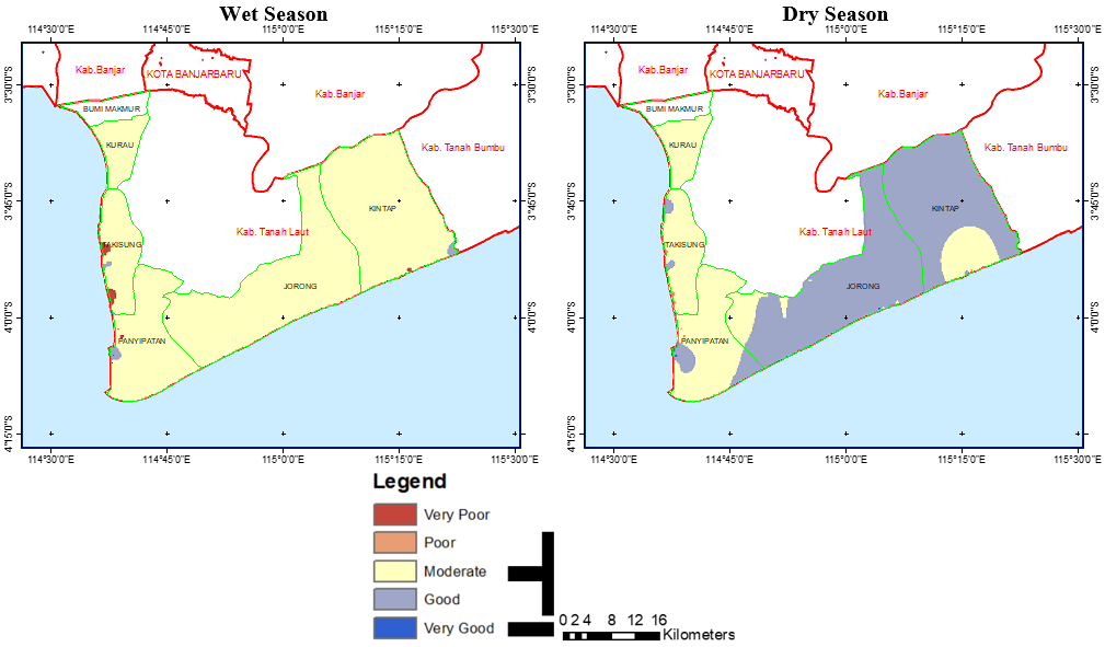
Field research revealed that wells are shallow and relatively close to septic tanks. Furthermore, the distance between houses is quite dense. Spatial analysis, shown in the map, also revealed a correlation between residential density and E. coli contamination levels. Areas with high domestic activity density tended to exhibit consistently lower water quality levels across both seasons. These findings align with research findings [59], which stated that exposure to E. coli contamination in clean water is significantly influenced by sanitation conditions and community behavior regarding domestic waste management.

Thus, the interpretation of these research results confirms that E. coli contamination in well water in the coastal area of Tanah Laut is a multidimensional phenomenon influenced by seasonal variability and community sanitation. A partial management approach will not be effective in reducing the risk of contamination, requiring an integrated strategy that includes protecting water sources, improving sanitation systems, and continuous spatial and temporal monitoring of water quality.

Table 5. Seasonal comparison of nutrient concentrations in matched wells

3.3 Relationship between agricultural land distance and groundwater quality parameters

The relationship between groundwater quality and agricultural land was evaluated using the distance from each well to the nearest agricultural land boundary, rather than distance to the centre of agricultural fields. The distance was calculated in a GIS environment using the recorded well coordinates and the mapped agricultural land-use layer. The land-use map added to the Results section shows that residential areas in the coastal sub-districts are spatially close to rice fields, plantation areas, and coastal aquaculture ponds. This spatial configuration indicates that many domestic wells are located within settlement areas that are directly adjacent to agricultural and pond-based production activities. Therefore, the variable is described as proximity to agricultural land, not direct fertilizer exposure (Figure 2).

Field observations also indicated that the coastal communities in the study area are commonly engaged in farming and aquaculture-related livelihoods. Both activities may involve the use of nitrogen- and phosphorus-containing inputs, including fertilizers and pond management materials. However, because no farm-level fertilizer application records were available, the analysis does not quantify fertilizer exposure directly. Instead, agricultural proximity is used as a spatial indicator of potential influence from nearby cultivated land and aquaculture-associated activities.

Because the nutrient variables and paired seasonal differences were not normally distributed, the association between agricultural land proximity and groundwater quality parameters was evaluated using Spearman’s rank correlation. All analyses were conducted using the 50 matched wells sampled in both wet and dry seasons. The spatial associations between proximity to agricultural land and groundwater nutrient concentrations in both seasons are summarized in Table 4.

Distance from agricultural land showed a negative association with nitrate concentration in both seasons, although the relationship was not statistically significant at the 0.05 level. In the wet season, nitrate showed a weak negative correlation with distance from agricultural land boundary (Spearman’s ρ = -0.262, P = 0.066, 95% CI: -0.524 to 0.037). A similar pattern was observed in the dry season (ρ = -0.255, P = 0.074, 95% CI: -0.504 to 0.027). These findings suggest a tendency for wells located closer to agricultural land to have higher nitrate concentrations, although the statistical evidence was not sufficient to confirm a significant spatial association.

Ammonia showed weak and non-significant correlations with agricultural distance in both seasons. The correlation was very weak in the wet season (ρ = -0.080, P = 0.583, 95% CI: -0.352 to 0.211) and remained non-significant in the dry season (ρ = -0.205, P = 0.154, 95% CI: -0.465 to 0.067). This indicates that ammonia variability was not primarily explained by proximity to agricultural land. Instead, ammonia concentrations may be influenced by localized processes, including organic matter decomposition, microbial transformation, domestic wastewater inputs, and well-specific environmental conditions.

The strongest and most consistent spatial relationship was observed for phosphate. Phosphate concentration was strongly and inversely correlated with distance from the agricultural land boundary in both the wet season (ρ = -0.943, P = 1.41 × 10⁻²⁴, 95% CI: -0.971 to -0.878) and dry season (ρ = -0.889, P = 6.73 × 10⁻¹⁸, 95% CI: -0.953 to -0.776). These results indicate that wells located closer to agricultural land consistently had higher phosphate concentrations. The spatial pattern is consistent with the land-use map, which shows that settlement areas and domestic wells are located near agricultural and aquaculture areas. Thus, phosphate enrichment in shallow groundwater may be related to the proximity of wells to land-use activities that commonly involve phosphorus-containing inputs, although direct fertilizer loading was not measured in this study.

Overall, the results show that proximity to agricultural land was most strongly associated with phosphate concentrations, while nitrate showed only a weak and non-significant tendency and ammonia showed no clear spatial pattern. These findings suggest that agricultural land proximity is an important spatial indicator for assessing groundwater nutrient risk, particularly for phosphate, but should not be interpreted as direct evidence of fertilizer exposure without supporting fertilizer application data.

Seasonal comparisons of nitrate, ammonia, and phosphate concentrations in the 50 matched wells are presented in Table 5. Because the paired differences were not normally distributed, the Wilcoxon signed-rank test was used as the primary seasonal test. Nitrate had a higher mean concentration in the dry season than in the wet season; however, because the distribution was skewed, the Wilcoxon signed-rank test was used as the primary test. The paired comparison indicated a significant seasonal shift in nitrate concentrations (W = 171.0, P = 0.006458, rank-biserial correlation = -0.514), with a median paired difference of -0.270 mg/L for dry minus wet season values. The median paired difference of −0.270 mg/L was calculated from the dry-minus-wet difference within each matched well and is therefore not equivalent to the difference between the overall seasonal medians. The apparent difference in direction reflects the skewed distribution of the paired changes and the influence of several relatively large dry-season nitrate values on the overall mean.

Ammonia increased in mean concentration from the wet season to the dry season, but the paired seasonal difference was not statistically significant (W = 78.0, P = 0.192199, rank-biserial correlation = 0.325). The median paired difference was 0.000 mg/L, indicating that most wells showed little seasonal change in ammonia concentration.

Phosphate showed a clear seasonal decrease from the wet season to the dry season. The Wilcoxon signed-rank test confirmed a significant seasonal difference (W = 0.0, P = 2.41 × 10⁻⁷, rank-biserial correlation = -1.000), with a median paired difference of -0.277 mg/L for dry minus wet season values. This indicates that phosphate concentrations were consistently higher during the wet season, suggesting that rainfall-driven runoff and leaching from agricultural land may enhance phosphate transport into shallow groundwater.

Overall, the results indicate that phosphate was the nutrient most strongly associated with proximity to agricultural land and showed a significant seasonal response. Nitrate showed a weak negative relationship with agricultural distance and a statistically significant seasonal shift, but the direction of seasonal change should be interpreted carefully because mean and paired-rank patterns differed. Ammonia showed no clear spatial or seasonal pattern, suggesting that its concentration was more likely influenced by localized well conditions and biogeochemical processes than by agricultural distance alone.

3.4 Distribution of E. coli contamination in groundwater

E. coli contamination was evaluated as a microbiological indicator of fecal contamination in the 50 matched domestic wells sampled during the wet and dry seasons. Because the drinking-water requirement for E. coli is zero detection in a 100 mL sample, any detectable E. coli concentration was classified as microbiologically non-compliant. The uploaded dataset includes well depth, distance to sanitation facilities, distance to the coast, sub-district location, and wet- and dry-season E. coli concentrations for all 50 wells.

The descriptive results show that E. coli contamination was widespread in both seasons, although concentrations were generally higher during the wet season. In the wet season, E. coli was detected in 48 of 50 wells, equivalent to 96.0% of samples. Concentrations ranged from 0 to 201, with a mean of 68.18 ± 58.01 and a median of 60.0. In the dry season, E. coli was detected in 44 of 50 wells, equivalent to 88.0% of samples. Dry-season concentrations ranged from 0 to 190, with a mean of 53.16 ± 54.97 and a median of 37.5. These results indicate that most wells did not meet the zero-detection requirement in either season, although both the proportion of positive wells and the median concentration were lower in the dry season. The seasonal and sub-district distributions of E. coli-positive wells, descriptive concentrations, and compliance with the zero-detection standard are summarized in Table 6.

Sub-district patterns showed that E. coli contamination occurred across all coastal areas, but the magnitude varied. Takisung showed consistently high contamination, with all sampled wells positive in both seasons and median values of 72.5 in the wet season and 50.0 in the dry season. Kurau and Kintap also showed complete or near-complete detection across seasons, although their median concentrations were lower than those in Takisung. Panyipatan had the lowest proportion of E. coli-positive wells, decreasing from 8 of 10 wells (80.0%) in the wet season to 7 of 10 wells (70.0%) in the dry season. Accordingly, two wells met the zero-detection requirement in the wet season, compared with three wells in the dry season. In Jorong, all wells were positive in the wet season, but three wells met the zero-detection requirement during the dry season.

4.png

Figure 4. E. coli contamination map in clean water wells