Atheer Saleem Almawla![]() | Basheer Al-Hadeethi*
| Basheer Al-Hadeethi*![]() | Ahmed Saud Mohammed
| Ahmed Saud Mohammed![]() | Ammar Hatem Kamel
| Ammar Hatem Kamel![]()
© 2024 The authors. This article is published by IIETA and is licensed under the CC BY 4.0 license (http://creativecommons.org/licenses/by/4.0/).
OPEN ACCESS
For thousands of years, people have understood the importance of evapotranspiration (ET) in maintaining the hydrologic cycle and replenishing the world's freshwater supplies. The process of estimating evapotranspiration with a high accuracy in arid regions is considered one of the most important processes in hydrological studies. It has a great importance in the efficient management of water resources and hydrological modeling, as well as in the management of irrigation operations, because these areas are permanently linked to the issue of water scarcity. The prediction of evapotranspiration is a vital step towards management of water resource. This study aims to develop an artificial neural network model to predict the evapotranspiration in arid regions. The RBFNN and GRNN models with six input data were used in present study. The input data are Max. temperature, Min. temperature, Ava. Temperature, Humidity, Wind speed and Solar radiation. The ANN modelling was achieved by using MATLAB with hyperbolic sigmoid transfer function for both input and output layers. Several statistical indicators have been used for examining the model's prediction accuracy. Results show that the current model is a powerful model which has the capability to predict the evapotranspiration with high accuracy. The superiority of the GRNN model is very obvious in comparison to the RBFNN model, where the coefficient of determination for GRNN model was more than 96% in comparison with 94% for RBFNN and the mean square error for GRNN was 0.4 in comparison with 0.52 for RBFNN model.
evapotranspiration, artificial neural network, RBF, GRNN, prediction, sensitivity analysis
The hydrological cycle's second-most significant component is the evapotranspiration (ET). Evapotranspiration is defined as the process in which water leaves the Earth's surface and plant bodies as vapor, then reaches the atmosphere. It is considered one of the most important calculations of the water balance in arid and semi-arid environments [1, 2]. It must be accurately estimated for different reasons which include: climate research, water balance, and water management in various agricultural activities [3-5].
Huge efforts from researchers, to introduce different studies to manage water resources have been achieved. Large number of such studies interested in the hydrological cycle parameters mostly the water losses that resulted from the evapotranspiration at the arid and semi-arid regions [6]. Since direct measurement of the rate of evapotranspiration is challenging and the process is imperceptible, number of models have been introduced to estimate it, based on the meteorological data that were collected under various climatic circumstances [7]. The physical-based complicated Penman-Monteith (PM) equation using full meteorological data is the only suggested approach for ET estimation [8, 9]. For many years, one of the main issues in hydrology was how to measure transpiration from various types of plants and evaporation from open water surfaces. The method that was used for detecting evaporation is called X, and it might not be accessible in certain climate stations. If it is, evaporation measurements could occasionally be unreliable because of things like improper maintenance or algae development within the tank [10]. Most studies indicate that the interrelationships that explain the occurrence of the process of evapotranspiration and the factors affecting its occurrence are unclear and non-linear [11]. The capability of artificial intelligence to mimic human brain functions gives it the ability to manage and understand complex problems and situations [7, 11, 12].
Due to the importance of the evapotranspiration process, especially in dry areas where water resources are scarce, this study emerged in an attempt to create a predictive mathematical model using artificial neural networks and devise a predictive equation which is lacking in the study area for estimating the quantities of water losses, resulting from evapotranspiration by identifying the climate variables that control the evapotranspiration process and use them as input to the predictive model
Recently, Abo El-Magd et al. [13] employed climate data from the weather station in Kafr El-Sheikh zone as inputs, in addition to the reference evapotranspiration values which were calculated through the Penman method - Monteith equation (PM), to develop a predictive model for evapotranspiration (ET). Seven different ANN models were trained and tested using the datasets. These models include various combinations of five diurnal meteorological variables which are: precipitation (P), wind speed (u), maximum and minimum air temperature (Tmax and Tmin), and dew point temperature (Tdw). The optimization method was a feedforward multi-layer artificial neural network. For the purpose of creating the final structure, Tansigmoid transfer function with the structure 1-5-6 was used. The study showed that adding the time indicator as an input to all groups greatly improved the process of predicting ETo values, and that involving the rainfall component as a variable had no effect on the network’s performance.
Patel et al. [14] predicted weekly reference evapotranspiration (ETo) in Sikkim region, India using multiple linear regression (MLR) method and artificial neural network (ANN).
The Penman Monteith method was used to estimate the value of ETo based on daily meteorological data for the period from 1985 - 2009. To develop the ANN and MLR model, based on the data set, several different sets of meteorological parameters were created. For the purpose of examining the efficiency of the models that were developed using ANN and MLR, several performance indicators were used, such as the coefficient of determination (R2), root mean square error (RMSR), mean absolute relative error (MAPE), mean absolute error (MAE), and Nash-Sutcliffe efficiency (NSC).
This study concluded that using a smaller number of meteorological variables and additional parameters increases the prediction efficiency of ANN and MLR models. Üneş et al. [5], estimated daily evapotranspiration (ET) using the Penman-Monteith equation and the classical Hargrens-Samani-Turk equation and compared the results with an artificial neural network (ANN) model in Lake Hartwell - USA. Relative humidity (RH), wind speed (U), solar radiation (SR), average daily air temperature (T), and maximum and minimum daily air temperatures (Tmax, Tmin) were used. An artificial neural network with feed forward and feedback was used to build the model. The study concluded that the performance of the ANN model in estimating daily ETo is better than other models. An analysis of the empirical equations and the ANN model reveal that the ANN model performs better than the other models in estimating daily ET.
Ali and Faraj [10] used the Penman-Monteith equation to estimate total daily evapotranspiration by calculating water loss by daily evaporation using data from 22 climate stations in Iraq for period of time from 2004 to 2013. The correlation coefficient is strong, according to the results. This study offered and suggested a technique to use the computed evaporation value, to determine the amount of evaporation for missing data for climatic stations in Iraq. The distribution of transpiration and evaporation in Iraq is illustrated in GIS maps. In their work, Pakhale et al. [15] estimated the daily evapotranspiration (ET) of reference grass crops by utilizing ANNs. Performance indicators were utilized to determine the performance of ANNs and traditional Penman-Monteith models, which were utilized for calculating ET. Using the MARS tool and the trial-and-error methodology that produced the best error statistics, and based on the above. Therefore, the input parameters and ANN model structure were chosen. Different ANN structures including BPNN, RBFNN and GRNN were employed. The results of the model indicates that the BPNN architecture is suitable for predicting the evapotranspiration of reference crops. Later, Aghelpour et al. [16] used machine learning techniques to estimate the daily evapotranspiration by utilizing an indirect method. Three meteorological stations were used for collecting seven daily meteorological variables from 2003 to 2016. To estimate the evapotranspiration, different techniques such as: Group Method of Data Handling (GMDH), Generalized Regression Neural Network (GRNN), Multilayer Perceptron (MLP), Radial Basis Function (RBF) were utilized. It was found that the GMDH model produced the best estimation, compared to the other models.
On the other hand, Bidabadi et al. [17] introduced a new model that was built utilizing the artificial intelligence to predict the evapotranspiration in Iran which has an arid region. To achieve this goal, they employed different techniques such as: ANN-gray wolf optimization (ANN-GWO), fuzzy neural adaptive inference system (ANFIS), and artificial neural network (ANN). They found that the ANFIS produces the best estimation for the ET.
Recently, Aly et al. [18] used super learning techniques to estimate the evapotranspiration. This technique is used when there is a lack in data. Four machine learning technique models were employed in the study which are: K-Nearest Neighbor, AdaBoost Regression, Support Vector Regressor, and Extra Tree Regressor. It is found that the model has a high performance in predicting the ET.
Despite the good estimation of the mentioned models, these models are not applicable in the region of the current study which has different climatic circumstances and for the limited meteorological information in this region.
The objective of current study is to demonstrate the feasibility of ANN techniques in modeling daily reference ET using climatic parameters in the arid area, Ramadi city in Iraq.
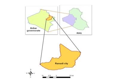
Ramadi city, within Anbar province, is located at the western part of Iraq. It was chosen as a study area, as shown in Figure 1. Little rainfall, high temperatures, low relative humidity and a significant difference between day and night temperatures are the most important features of climate of this area. The maximum temperature may exceed 50℃ during summer, while it may decline to reach 9℃ during winter. The average annual evaporation may reach 3000 mm. The dryness coefficient, that represents the evaporation divided by rain, ranges from 25 to 35 [19]. In the present study, the climatic data for time period from 23/11/2020 to 1/10/2022, were utilized to predict the evapotranspiration. This data is collected from the digital meteorological station that was installed at the Upper Euphrates Basin Developing Centre at the University of Anbar, Ramadi, Iraq. The station, which has 50 m altitude above mean sea level, is located at 33.43° N latitude and 43.33° E longitude. The daily climatic data includes: evapotranspiration, wind speed, minimum temperature, maximum temperature, average temperature, relative humidity, and solar radiation.
Figure 1. The area under study
The design of ANNs was inspired by the brain's neural system. The majority of ANN models include three layers: the input layer that provides data for the model, the hidden layer which represents the detector for the input parameters characteristics and the output layer that reflects the model's reaction to specific inputs. In present study, two methods of artificial intelligence were used for modelling the evapotranspiration in arid region. The introduced models are simple to apply, time saving while producing results, and have a significant accuracy in prediction in the scope of hydrology.
3.1 Radial basis function neural network (RBFNN)
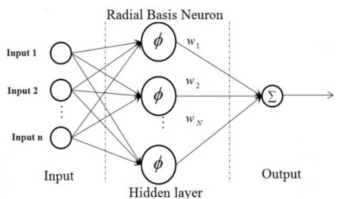
Figure 2. General architecture of a RBFNN [20]
Powell [20] was the first to introduce the RBFNNs for solving the interpolation problem in a multidimensional space with as many centers as data points. RBFNNs are based on a concept of function approximation. The interesting feature of RBFNNs, is the presence of the linear learning algorithm that is rapidly built in the network, which is able to model complicated non-linear mapping. RBFNNs are currently being investigated in numerical analysis and involved in machine learning techniques. The Euclidean distance from the point being evaluated to the center of each neuron is estimated, and a radial basis function (RBF) is applied to the distance, to determine the influence for each neuron. As shown in Figure 2, a radial basis function neural network consists of a three-layers network. The layers include: input layer, hidden layer and output layer.
The input layer can include several predictor variables, which are connected to the independent neurons in the hidden layer. Multiple input vectors were propagated from the input layer to the hidden layer. The hidden layer includes a number of radial basis function units $(n h)$ with Gaussian kernels and bias $\left(b_k\right)$. The $\mathrm{j}$-th Gaussian function is determined by a center $\left(c_i\right)$ and a width $\left(\sigma_j\right)$ [21]. The distance between the input vector ( $\mathrm{x}$ ) and the Gaussian function center ($c_j$), Euclidean distance, is calculated by the RBFNN classifier, then the nonlinear transformation is conducted in the hidden layer as presented in Eq. (1) bellow:
$h_i(x)=\exp \left(-\left\|x-c_i\right\|^2 / \sigma_i^2\right)$ (1)
where, $h_i$ represents the output of the $\mathrm{j}$-th neuron in the hidden layer. On the other hand, the linear operation of the output layer is shown in the following equation:
$y_k(x)=\sum_{j=1}^{n h} w_{k j} \cdot h_j(x)+b_k$ (2)
where, $y k$ represents the $\mathrm{k}$-th output unit for the input vector $x, w_{k i}$ represents the weight connection that links the j-th hidden layer unit and the $\mathrm{k}$-th output unit, and $b_k$ represents the bias. So, weights $\left(w_{k 1}, w_{k 2}, \ldots, w_{k n h}\right)$ are associated with each neuron in the output layer. The value output of a singular neuron in each hidden layer is multiplied by the weight associated with the neuron and transferred to the summation, which sums up the weighted values and displays the sum as the network's output. The bias value has been multiplied by a weight $b_k$ and provided into the output layer.
3.2 Generalized regression neural network
The generalized regression neural network (GRNN) is a variant to radial basis neural networks. It is proposed by Specht in 1991 [22]. It can be used for prediction, classification, and regression. GRNN is an enhanced approach which is built based on nonparametric regression. The training sample, in GRNN, represents a mean to a radial basis neuron. GRNN has a high accuracy in the estimation with using single pass learning, therefore it does not require backpropagation [23]. The GRNN can be mathematically represented by the following equation:
$Y(x)=\frac{\sum_{k=1}^N y_k K\left(x, x_k\right)}{\sum_{k=1}^N K\left(x, x_k\right)}$ (3)
where, Y(x) is the prediction value of input x, K(x, xk) is the Radial basis function kernel (Gaussian kernel)and yk is the activation weight for the pattern layer neuron at k.
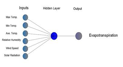
RBFNN and GRNN models have been used for predicting the evapotranspiration in Ramadi city. MATLAB 2020 Ra software was employed to analyze the evapotranspiration data. The Max temperature, Min temperature, Avar. Temperature, Humidity, Wind speed and Solar radiation were used as input for ANN parameters. The hidden layer of the RBFNN has a structure of six neurons, while it is one neuron for hidden layer of the GRNN model. The structure of the neural network model was found by applying the trial and error concept. Figure 3 illustrates the architecture of ANN model.
Figure 3. Architecture for generalized regression neural network (GRNN) method
For ANN modelling purposes, many functions can be used. By trial and error, the best transfer function equation for present model was TANCH (Hyperbolic Tangent) for both input and output layers. Levenberg–Marquardt backpropagation (trainlm) technique was utilized in the present paper, which is recommended for most cases [24]. To get the optimum generalization, the dataset should be divided into three parts: training, validation, and test. In present study, the input data was split into three sets. The first one is the training set which represents 70% of data. The second and third sets took up to 15% for both test and validation sets.
The training dataset is utilized to train the model by reducing the error of this dataset during training. The validation dataset is used for evaluating the performance of a neural network on patterns that were not trained. The tested dataset is used for assessing the overall performance of a trained and verified network [25].
The dimension variables must be eliminated to ensure that equal attention is required for each variable during training, which can be realized by scaling of all variables before training. The variables scaling depends on the output transfer function. The scaling of inputs and outputs data will have unity standard deviation and zero mean [26]. The data of present model was scaled based on the output transfer function (TANCH) by using the following equation:
$X_n=\frac{2\left(X-X_{\min }\right)}{X_{\max }-X_{\min }}-1$ (4)
where, Xn is the scaling value, X is the raw value, Xmax is the maximum value, and Xmin is the minimum value.
After completing the modeling, Performance evaluation criteria are used for checking the model's accuracy depending on the validation. By estimating the relation between the observed and the predicted data the accuracy will be achieved. In present study, four well-known metrics: RMSE, MAE, RE, and R2 were used for assessing the performance of the two models.
One of the most important criteria for selecting models is the test samples. Test set is the set of data that used for evaluating the final performance of a trained model. It serves as an unbiased measure of how well the model generalizes to unseen data, assessing its generalization capabilities in real-world scenarios. By keeping the test set separate throughout the development process, we obtain a reliable benchmark of the model’s performance.
The test dataset also helps gauge the trained model's ability to handle new data. Since it represents unseen data that the model has never encountered before, evaluating the model fit on the test set provides an unbiased metric for its practical applicability. This assessment enables us to determine if the trained model has successfully learned relevant patterns and can make accurate predictions beyond the training and validation contexts.
5.1 Descriptive analysis
The fundamental characteristics of the datasets in the current study, such as the minimum, maximum, mean, and standard deviation for the meteorological parameters' dataset, were described using descriptive statistics.
The ET data ranged from 0.33 mm to 13.8 mm with mean 5.46 mm, Max Temp ranged from 9.10℃ to 48.10℃ with mean 26.95℃ while Min Temp. ranged from -1.7℃ to 33.60℃ with mean 14.31℃. Table 1 depicts the descriptive statistics of meteorological.
Table 1. Descriptive analysis for meteorological parameters dataset
|
Parameters |
Minimum |
Maximum |
Mean |
Std. Dev |
|
ET |
0.33 |
13.80 |
5.46 |
2.78 |
|
Max_Temp |
9.10 |
48.10 |
26.95 |
9.12 |
|
Min_Temp |
-1.70 |
33.60 |
14.31 |
8.06 |
|
Av_Temp |
3.95 |
40.75 |
20.64 |
8.50 |
|
RH |
11.48 |
96.06 |
40.64 |
17.13 |
|
WS |
0.70 |
7.22 |
2.81 |
1.23 |
|
Solar_Rad |
18.25 |
316.92 |
182.05 |
68.55 |
5.2 Correlation matrix
Creating a correlation matrix is a statistical method that is used for assessing the relationship between two variables in records of a dataset. Each cell in the matrix table has a correlation coefficient. The correlation coefficient has a value equal to (1) for strong association, while (0) value represents a neutral relationship, and (-1) value represents a weak relationship between the variables.
Table 2 shows a strong positive correlation between ET and Solar_Rad, Max_Temperature, Min_Temperature and a negative relationship between ET and relative humidity. Meanwhile, there was a moderate relationship between ET and WS. Furthermore, the table also shows that there are strong relationships between independent variables, such as the relationship between Max_Temp, Min_Temp and Avar_Temp. In addition to the above, there are weak relationships between temperatures with wind speed.
Table 2. Pearson’s correlation coefficient between ET and other meteorological parameters
|
Parameters |
ET |
Max_Temp |
Min_Temp |
Av_Temp |
RH |
WS |
Solar Radiation |
|
ET |
1 |
0.860** |
0.838** |
0.858** |
-0.840** |
0.570** |
0.863** |
|
Max_Temp |
0.860** |
1 |
0.955** |
0.990** |
-0.810** |
0.220** |
0.726** |
|
Min_Temp |
0.838** |
0.955** |
1 |
0.987** |
-0.733** |
0.318** |
0.655** |
|
Av_Temp |
0.858** |
0.990** |
0.987** |
1 |
-0.783** |
0.270** |
0.701** |
|
RH |
-0.840** |
-0.810** |
-0.733** |
-0.783** |
1 |
-0.312** |
-0.731** |
|
WS |
0.570** |
0.220** |
0.318** |
0.270** |
-0.312** |
1 |
0.305** |
|
Solar_Rad |
0.863** |
0.726** |
0.655** |
0.701** |
-0.731** |
0.305** |
1 |
5.3 Validation of model accuracy
The model's performance must be evaluated to investigate the capability of the model to achieve an accurate estimation of the evapotranspiration. Some statistical directories can be used for examining the output of model against the actual records of the evapotranspiration value. In the present model the statistical directories such as Mean Absolute Error (MAE), Root Mean Square error (RMSE), relative error (RE), and coefficient of determination (R2) were used. The following equations were utilized to calculate the performance criterion of models between output and the measured values. Table 3, demonstrates the measured statistical directories for the present model. The value of statistical directories in Table 3 with coefficient of determination values shows that the model has a high accuracy with a very strong positive relationship between measured and predicted values. For all statistical indicators in Table 3, the GRNN model outperformed on the RBFNN model in the prediction of ET. This is clear in the value of RMSE, MAE, RE and R2 for two models. Below are the equations that were used in the calculation of statistical directories [27].
$R M S E=\sqrt{\frac{1}{N}} \sum_{i=1}^N\left(M_i-P_i\right)^2$ (5)
$M A E=\frac{1}{N} \sum_{i=1}^N\left|M_i-P_i\right|$ (6)
$R E=\left[\frac{\left|P_i-M_i\right|}{M_i}\right] \times 100$ (7)
where, Mi is the measurements, Pi is the predicted value.
Table 3. The statistical directories for the model
|
Statistical Directories |
MAR |
RMSE |
RE |
R2 |
|
GRNN mode |
0.406 |
0.61 |
9.87% |
96.8% |
|
RBFNN model |
0.52 |
0.717 |
11.42% |
94.2% |
5.4 The measured and predicted relationship
The data that was recorded at the meteorological station for about 540 days were employed in present model. This data was utilized to ensure the ability of the ANN model for prediction of daily evapotranspiration. The ANN is used for identifying the relation between observed values and predicted values, which is based on the number of hidden layer nodes and transfer functions. The best models are selected based on the idea of trial and error by continuous training to obtain the best value of coefficient of determination (R2) in the test stage with the smallest error, indicating that the best prediction performance has been achieved. By trial and error, the optimal structure of GRNN and RBFNN model was one hidden layer and three hidden layers, respectively.
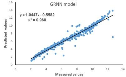
Figure 4. The scatter plot between measured – predicted evapotranspiration for GRNN model
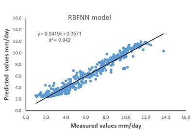
Figure 5. The scatter plot between measured – predicted evapotranspiration for RBFNN model
The (R2) value between measured and predicted values was 98.3% and 97% for GRNN and RBFNN model, respectively. Figure 4 and Figure 5 illustrate the scatter plot between the predicted and measured values for the two forementioned models.
The GRNN and RBFNN models with six inputs data of climatic were utilized to predict the evapotranspiration. The results demonstrated that the GRNN and RBFNN models were able to predict ET with high accuracy. A nonlinear equation has been found that can be utilized to predict daily evapotranspiration. This equation represents the first model for determining the evapotranspiration in the study area. the new equation is very useful for calculating the losses of evapotranspiration in Ramadi city, which contributes to the management of water resources in the city.
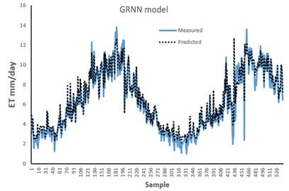
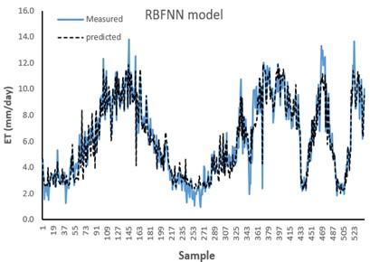
On the other hand, the relation between measured and predicted values for both models can be shown in Figure 6 and Figure 7. In these figures, a high convergence between measured ET and predicted ET can be noted for both models.
Figure 6. The measured and predicted evapotranspiration for GRNN model
Figure 7. The measured and predicted evapotranspiration for RBFNN model
5.5 Sensitivity analysis
To investigate the input elements and find the element that has the most effect on evapotranspiration, the modified Garson algorithm method has been used. This method is used for determining the relevance of input elements. It is simple to be used for determining the relative relevance of every single element inside a network by dividing the neural network link's output weights [28]. The algorithm specifics are shown in the equation below.
$Q_{i k}=\frac{\sum_{j=1}^L\left|w_{i j} v_{j k}\right| / \sum_{r=1}^N\left|w_{r j}\right|}{\sum_{i=1}^N \sum_{j=1}^L\left(\left|w_{i j} v_{j k}\right| / \sum_{r=1}^N\left|w_{r j}\right|\right)}$ (8)
where,
- $Q_{i k}$ is the percent of input variable effect on output.
- $w_{i j}$ is the weight of a connection between input neuron i and hidden neuron j.
- $v_{j k}$ is the weight of the connection between hidden neuron j and output neuron k.
- $\sum_{r=1}^N\left|w_{r j}\right|$ is the weighted connection sum between the N input neurons and the hidden neuron j.
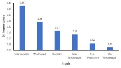
Figure 8 demonstrates the sensitivity analysis and the relevance of the input elements on the evapotranspiration losses.
Figure 8. Importance of input factors on evapotranspiration
Figure 8 illustrates that the most important input factors to determine the evapotranspiration losses are the solar radiation and wind speed - their importance exceeds 60%. The influence of humidity (17%) followed by Maximum temperature (13%) have the second significance effect to determine the evapotranspiration losses. From the results of sensitivity test of the model, the solar radiation and wind speed can clearly have an effect on the evapotranspiration losses. A slight increase in solar radiation and wind speed can lead to an increase in evapotranspiration. On the other hand, the average and minimum temperatures have no impact on the evapotranspiration. Undoubtedly the results of sensitivity analysis of the present model between the evapotranspiration losses and six aforementioned parameters varies from one region to another, according to the condition of the study area.
5.6 ANN model equations
Due to the importance of the evapotranspiration process in water resource management, especially in arid regions where water resources are scarce, this study developed a predictive mathematical model using artificial neural networks technique and devised a predictive equation that is lacking in the study area for estimating the quantities of water losses resulting from evapotranspiration.
The optimal ANN model, which is obtained based on a low number of connection weights, enables each network to be presented into a simple formula [29]. According to the threshold levels, connection weights, and transfer function the following equation can be employed to predict the equation between input parameters and output:
$I j=\sum I_i W_{j i}+\theta$ (9)
$X=\sum W_{k j} * T A N H(I j)$ (10)
$O=T A N H(X)$ (11)
where, $i=1,2,3, \ldots, 9,10$ (nodes in the input layers), $j=1,2,3$, $4, \ldots 12,13$ (nodes in the output layers), $k=1$ (output layer node), $W_{j i}$ and $W_{k j}$ are training weights given in Table 2 and Table 3. $I_i=$ Inputs, $\theta=$ bias. $O=$ predicted outputs.
The predicted evapotranspiration is expressed as follows:
$E T=6.405 *(T A N H(X))+7.395$ (12)
$X=20612.5883 * T A N H(H)+20609.3052$ (13)
$\begin{gathered}H=0.00204 * X_1-0.00042 * X_2+0.00094 * X_3- \\ 0.0013 * X_4+0.02178 * X_5+0.00041 * X_6-4.9264\end{gathered}$ (14)
where, X1 = Max temperature (℃), X2= Min temperature (℃), X3= Ava. Temperature (℃), X4= Humidity (%), X5= Wind speed (m/s), X6= Solar radiation (w/m2).
The equations above are based on identifying the climate variables, controlling the process of evapotranspiration and using it as an input to the predictive.
The artificial neural network has a high capability of predicting the evapotranspiration. Developing an equation can be employed to predict the daily evapotranspiration losses in arid regions. According to the sensitivity analysis of the data, the solar radiation and wind speed have the most influence on evapotranspiration followed by humidity and maximum temperature. On the other hand, the average and minimum temperatures have an unnoticeable effect on the evapotranspiration losses. According to the statistical criteria and coefficient of determination, the GRNN model outperforms the RBFNN model in predicting the evapotranspiration. According to the findings of this study, the GRNN model is a very useful tool for calculating evapotranspiration. The sensitivity analysis shows that solar radiation and wind speed are more important input factors of evapotranspiration. The neural network technology that was employed in this paper can be widely used in improving water resources management. By understanding the elements of the hydrological cycle, more effective and practical decisions can be made in managing available resources and reducing evapotranspiration. The importance of the current study comes from the fact that the study area lacks data and scientific research in this field. In addition to availability of few numbers of weather stations.
[1] Sha, J.X., Liu, B., Wang, S.Q., Liang, L.J. (2012). Water resources management based on the ET control theory. Procedia Engineering, 28: 665-669. https://doi.org/10.1016/j.proeng.2012.01.788
[2] Deus, D., Gloaguen, R., Krause, P. (2013). Water balance modeling in a semi-arid environment with limited in situ data using remote sensing in Lake Manyara, East African Rift, Tanzania. Remote Sensing, 5(4): 1651-1680. https://doi.org/10.3390/rs5041651
[3] Makwana, J.J., Tiwari, M.K., Deora, B.S. (2023). Development and comparison of artificial intelligence models for estimating daily reference evapotranspiration from limited input variables. Smart Agricultural Technology, 3: 100115. https://doi.org/10.1016/j.atech.2022.100115
[4] Patle, G.T., Singh, D.K. (2015). Sensitivity of annual and seasonal reference crop evapotranspiration to principal climatic variables. Journal of Earth System Science, 124: 819-828. https://doi.org/10.1007/s12040-015-0567-8
[5] Üneş, F., Doğan, S., Taşar, B., Kaya, Y., Demirci, M. (2018). The evaluation and comparison of daily reference evapotranspiration with ANN and empirical methods. Natural and Engineering Sciences, 3(3): 54-64.
[6] Chen, S.H., Jakeman, A.J., Norton, J.P. (2008). Artificial intelligence techniques: An introduction to their use for modelling environmental systems. Mathematics and Computers in Simulation, 78(2-3): 379-400. https://doi.org/10.1016/j.matcom.2008.01.028
[7] Mohammed, A.S., Al-Hadeethi, B., Almawla, A.S. (2023). Daily evapotranspiration prediction at arid and semiarid regions by using multiple linear regression technique at Ramadi City in Iraq region. In IOP Conference Series: Earth and Environmental Science, 1222(1): 012033. https://doi.org/10.1088/1755-1315/1222/1/012033
[8] Chen, D. (2012). Daily reference evapotranspiration estimation based on least squares support vector machines. In Computer and Computing Technologies in Agriculture V: 5th IFIP TC 5/SIG 5.1 Conference, CCTA 2011, Beijing, China, pp. 54-63. https://doi.org/10.1007/978-3-642-27278-3_7
[9] Iliadis, L.S., Maris, F. (2007). An artificial neural network model for mountainous water-resources management: The case of Cyprus mountainous watersheds. Environmental Modelling & Software, 22(7): 1066-1072. https://doi.org/10.1016/j.envsoft.2006.05.026
[10] Ali, H.Z., Faraj, S.H. (2017). Estimation of daily evaporation from calculated evapotranspiration in Iraq. Journal of Madenat Alelem University College, 9(2): 84-96.
[11] Mohammed, A.S., Almawla, A.S., Thameel, S.S. (2022). Prediction of monthly evaporation model using artificial intelligent techniques in the western desert of Iraq-Al-Ghadaf Valley. Mathematical Modelling of Engineering Problems, 9(5): 1261-1270. https://doi.org/10.18280/mmep.090513
[12] Rajanayaka, C., Samarasinghe, S., Kulasiri, D. (2002). Solving the inverse problem in stochastic groundwater modelling with artificial neural networks. In 1st International Congress on Environmental Modelling And Software, Lugano, Switzerland.
[13] Abo El-Magd, A., Baraka, S.M., Eid, S.F. (2023). Using artificial neural networks to predict the reference evapotranspiration. Journal of Water and Land Development, 57: 1-8.
[14] Patle, I.T., Mandal, B.P., Kumar, M., Jhajharia, D. (2022). Evapotranspiration modelling using artificial neural network and multiple linear regression approach in Semi-Humid Region of Sikkim. Journal of Agricultural Engineering. https://doi.org/10.21203/rs.3.rs-1598141/v1
[15] Pakhale, G.K., Nale, J.P., Temesgen, W.B., Muluneh, W.D. (2015). Modelling reference evapotranspiration using artificial neural network: A case study of Ameleke watershed, Ethiopia. International Journal of Scientific and Research Publications, 5(4): 1-8.
[16] Aghelpour, P., Bahrami-Pichaghchi, H., Karimpour, F. (2022). Estimating daily rice crop evapotranspiration in limited climatic data and utilizing the soft computing algorithms MLP, RBF, GRNN, and GMDH. Complexity, 2022(1): 4534822. https://doi.org/10.1155/2022/4534822
[17] Bidabadi, M., Babazadeh, H., Shiri, J., Saremi, A. (2024). Estimation reference crop evapotranspiration (ET0) using artificial intelligence model in an arid climate with external data. Applied Water Science, 14(1): 1-10. https://doi.org/10.1007/s13201-023-02058-2
[18] Aly, M.S., Darwish, S.M., Aly, A.A. (2024). High performance machine learning approach for reference evapotranspiration estimation. Stochastic Environmental Research and Risk Assessment, 38(2): 689-713. https://doi.org/10.1007/s00477-023-02594-y
[19] Al-Dabbas, M.A., Ayad Abbas, M., Al-Khafaji, R.M. (2012). Dust storms loads analyses—Iraq. Arabian Journal of Geosciences, 5: 121-131. https://doi.org/10.1007/s12517-010-0181-7
[20] Powell, M.J. (1987). Radial basis functions for multivariable interpolation: A review. Algorithms for Approximation, 143-167.
[21] Montazer, G.A., Giveki, D., Karami, M., Rastegar, H. (2018). Radial basis function neural networks: A review. Computer Reviews Journal, 1(1): 52-74.
[22] Specht, D.F. (1991). A general regression neural network. IEEE Transactions on Neural Networks, 2(6): 568-576.
[23] Kamel, A.H., Afan, H.A., Sherif, M., Ahmed, A.N., El-Shafie, A. (2021). RBFNN versus GRNN modeling approach for sub-surface evaporation rate prediction in arid region. Sustainable Computing: Informatics and Systems, 30: 100514. https://doi.org/10.1016/j.suscom.2021.100514
[24] Bui, X.N., Muazu, M.A., Nguyen, H. (2020). Optimizing Levenberg–Marquardt backpropagation technique in predicting factor of safety of slopes after two-dimensional OptumG2 analysis. Engineering with Computers, 36: 941-952. https://doi.org/10.1007/s00366-019-00741-0
[25] Zhang, G., Patuwo, B.E., Hu, M.Y. (1998). Forecasting with artificial neural networks: The state of the art. International Journal of Forecasting, 14(1): 35-62. https://doi.org/10.1016/S0169-2070(97)00044-7
[26] Aziz, J., R Mahmood, K. (2012). Using artificial neural networks for evaluation of collapse potential of some Iraqi gypseous soils. Iraqi Journal of Civil Engineering, 7(1): 21-28.
[27] Chai, T., Draxler, R.R. (2014). Root mean square error (RMSE) or mean absolute error (MAE)?–Arguments against avoiding RMSE in the literature. Geoscientific Model Development, 7(3): 1247-1250.
[28] Almawla, A.S., Lateef, A.M., Kamel, A.H. (2022). Modelling the effects of hydraulic force on strain in hydraulic structures using ANN (Haditha dam in Iraq as a case study). Mathematical Modelling of Engineering Problems, 9(1): 150-158. https://doi.org/10.18280/mmep.090119
[29] Al-Zubaidi, D.S., Aljanabi, K.R., Khaled, Z.S. (2024). Using artificial neural networks to estimate the unconfined compressive strength of gypseous soil. AIP Conference Proceedings, 2864(1): 030034. https://doi.org/10.1063/5.0186191