Forecasting CO2 Emissions in Malaysia Through ARIMA Modelling: Implications for Environmental Policy

Yogesswary Segar![]() | Noor Haslina Mohamad Akhir
| Noor Haslina Mohamad Akhir![]() | Nur Azura Sanusi*
| Nur Azura Sanusi*![]()
© 2024 The authors. This article is published by IIETA and is licensed under the CC BY 4.0 license (http://creativecommons.org/licenses/by/4.0/).
OPEN ACCESS
Carbon dioxide (CO2), a prominent constituent of greenhouse gases, has a vital impact on environmental pollution and the occurrence of global warming. Malaysia is categorised as the primary contributor to CO2 emissions among the ASEAN countries. Malaysia's total CO2 emissions had a significant increase, surging by a factor of nine, from 28 Mt in 1980 to 262.2 Mt in 2020. This indicates analysing the significance of CO2 emissions is an urgent concern in Malaysia. Therefore, the objective of this study is to forecasts the magnitude of CO2 emissions that will be discharged in Malaysia during a span of ten years, specifically from 2021 to 2030. This study utilises quantitative modelling, namely auto-regressive integrated moving average (ARIMA) analysis, to assess the yearly time series data of CO2 emissions in Malaysia spanning from 1970 to 2020. The findings reveal that Malaysia's CO2 emissions are expected to continue rising in the next ten years, albeit with a gradual decline. This finding contributes to the body of knowledge and provides Malaysian policymakers with an opportunity to strengthen their current economic and environmental policies. This, in turn, could help create a safer environment and mitigate the negative impacts of CO2 emissions.
ARIMA, CO2 emissions, Malaysia, forecasting, environment
Natural resources serve as fundamental building blocks in socio-economic systems at the local, regional, national, and global scales, playing a crucial role in shaping the well-being of humanity, the environment, and the economy [1]. However, the growing interdependence of diverse economies around the world has a variety of effects on the environment. Unlike any other period in human history, the current trend is marked by a rise in detrimental effects on the global environment, specifically in the form of an increase in heat-trapping gases [2, 3]. Human activities have undeniably played a significant role in the increase in the number of heat-trapping gases over the past decades. Especially carbon dioxide (CO2) which is a substantial heat-trapping (greenhouse) gas that is emitted by human activities like deforestation and the burning of fossil fuels, as well as through natural processes like breathing and volcanic outbursts [4]. If we look at global CO2 emissions, they rose from 20.5 billion metric tonnes in 1990 to 31.5 billion metric tonnes in 2020 [5]. The environment and people will not benefit from this rise.
Further, rising greenhouse gases, particularly CO2 emissions gas, are primarily responsible for climate change [6-8]. Again, this rising CO2 emissions from increased use of fossil fuels, rapid urbanisation, industrialization, transportation, and population growth [9, 10] cause the global mean temperature to rise. Therefore, over the years, climate change has gained more attention with frequent news coverage of extreme weather phenomena such as melting glaciers and heatwaves [11]. Malaysia is not exempt to this issue as evidenced by latest event in December 2021, eight states in Peninsular Malaysia were affected by severe flooding and severe rains that pounded the region's eastern coast. At least 54 people were killed, two are still missing, and 30,000 more were affected by Malaysia's worst flooding in years [12]. Malaysia since 1970s, has achieved remarkable global economic growth, resulting in a significant increase in per capita income. This rapid progress is primarily attributed to Malaysia's dominant role as a top exporter of both manufactured goods and primary commodities [13]. According to world bank, Malaysia’s per-capita income increased from 384 US dollars in 1971 to 10,412 US dollars in 2020 [14].
For developing economies like Malaysia, a high level of development is essential. However, when society and the economy transition from a low to a middle stage of development, it will lead to a decline in the country's environmental condition [15]. For example, when Malaysia underwent a rapid transition from an economy reliant on agricultural to one focused on industry, its CO2 emissions also sharply surged [15]. This is attributed to heightened global competition in pursuit of targeted economic growth, leading to increased resource and energy consumption and contributing to the deterioration of the country's environmental state [16]. Even the EKC theory stated that environmental issues are serious for nations in the early stages of development, especially for developing countries desiring to become developed [17]. According to Zaman et al. [18] and Tella et al. [19], Malaysia is ranked 117th out of 180 countries with the poorest air quality and CO2 emissions are 8.03 metric tons per capita, which represents the third highest after Brunei and Singapore [20, 21].
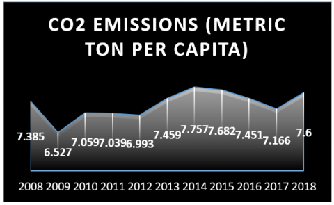
This is due to the pattern of nations' economic growth becoming more unsustainable and having difficulty in implementing climate action goals established by our government. Therefore, the air quality in Malaysia has worsened since the 1970s as the per capita emission of CO2 has risen [22], and Malaysia's ability to achieve a 40% reduction in emissions by 2020 has proven problematic [23]. Figure 1 illustrates a 10-year trend depicting the rise in Malaysia's overall CO2 emissions. In 2008, the country's CO2 emissions per capita were 7.385 metric tons, increasing to 7.6 metric tons in 2018. Despite a temporary decline of 6.527 metric tons per capita in 2009 due to an economic downturn, emissions rebounded the following year, rising by 7.059 metric tons. Notably, Malaysia witnessed significant carbon emissions between 2008 and 2018, peaking at 7.757 metric tons per capita in 2014. This surge in emissions can be attributed to Malaysia's economic development goals and increased production, leading to a worsening environmental situation. Particularly, the urban and industrial areas in peninsular Malaysia are major contributors to heavy pollutant emissions, as highlighted by Alyousifi et al. [24]. Malaysia, aspiring to achieve industrialized status soon [19, 25], faces challenges in balancing economic growth with environmental sustainability.
Figure 1. CO2 emission of Malaysia
Source: data retrieved from World Bank [26]
To curb the rise in global CO2 emissions, the United Nations' Sustainable Development Goals prioritize environmental protection. In pursuit of SDG 13, which focuses on combating climate change, the majority of nations are striving to implement policies, especially regulations, aimed at reducing CO2 emissions [27]. Malaysia is not an exception. Because Malaysia is one such developing nation that has undergone rapid economic growth in the past 40 years, resulting in a slew of environmental issues especially, the emission of CO2 [28]. Therefore, it is crucial to understand this region's CO2 emissions both present day and in the future. This rising degree of environmental degradation in Malaysia forms a pressing concern for analysts and decision-makers [29]. Thus, forecasting CO2 emissions will aid in raising public awareness and has become increasingly important for policymakers and researchers seeking to mitigate the adverse effects of climate change.
Besides, most of the surveyed literatures focused on applying specific time period using various approaches to predict CO2 emissions. For example, Sulaiman et al. [30] employed the Conventional Multivariable Grey Model (CMGM) approach, Shekarchian et al. [31] utilized energy analysis techniques, Tan et al. [32] employed Best Subsets Regression and Multi-Linear Regression, Pauzi and Abdullah [33] utilized a fuzzy inference system (FIS), and Kee et al. [34] applied multiple linear regression and trend analysis, among others. However, this study uses the ARIMA (Autoregressive Integrated Moving Average) models, specifically the Box-Jenkins methodology, to estimate and forecast future CO2 emissions in Malaysia over a ten-year period from 2021 to 2030. This change in methodology adds to the novelty and uniqueness of our paper, presenting an opportunity to gain fresh insights into the factors influencing CO2 emissions in the specific context of Malaysia. Furthermore, in comparison with existing models, we aim to provide a more nuanced and accurate assessment of future emissions trajectories. Through our efforts, this will provide a valuable contribution to the understanding of environmental dynamics in this region and offer insights that may inform sustainable policies and practices moving forward.
The Paris Agreement-Conference of Parties 21 (COP21), held in 2015, was a significant advancement in GHG emission reduction efforts. All parties provided commitments to reduce emissions countrywide [35]. The CO2 emissions have been forecasted in many countries because of their serious effects on the climate.
The study by Shekarchian et al. [31] focused on cost-benefit analysis and prospective assessment of emission reduction through the application of wall insulation in buildings in Malaysia. The study's principal aim is to forecast any prospective changes in emission production over a span of 20 years, using three distinct scenarios. For Scenario 1, it can be noted that rigid fibreglass has the lowest emission reduction rate, whereas fiberglass-urethane has the highest rate. However, their overall result for this scenario indicates that for the following 20 years, the rate of emission production dramatically rose. Based on the analysis of CO2 emissions in the second scenario, the fuel composition in Malaysia's power industry is expected to undergo a gradual change from 2012 to 2031. This change reflects a downward trend over the next two decades, primarily driven by the emission reduction policies implemented by major electricity providers in Malaysia. The third scenario's CO2 production values are based on the optimal thickness of various thermal insulators. According to their overall analysis of this scenario, emission production related to fiberglass-urethane will decline from 16.7 (kg/m2) in 2012 to 7.3 (kg/m2) in 2031.
Furthermore, the prediction models that evaluate and compute the CO2 emission in Malaysia are presented in the Tan et al. [32] study. The three primary categories of transportation, electricity, and residential will be used to examine each CO2 emission forecast model. Their combined finding for all three sectors demonstrates that CO2 emissions have increased and will likely continue to do so through 2021. Pauzi and Abdullah’s [33] research described Fuzzy inference system (FIS) to forecast CO2 emissions in Malaysia. Additionally, their FIS prediction results diverge significantly from the actual values and adaptive neuro-fuzzy inference system (ANFIS) prediction values. This indicates that the predicted value of CO2 differs from the measured value. For instance, the actual amount of CO2 emission in 2009 was lower than the amount predicted to be emitted that year. The study by Kee et al. [34] is to investigate how Nonintrusive load monitoring (NILM) affects CO2 emissions in Malaysia. Forecasting models for their studies were developed using open data from Malaysia from 1996 to 2018. According to their forecasting findings, Malaysia's overall CO2 emissions trend would continue to rise through 2030 without reaching a peak.
Mustaffa and Shabri [36] conducted a study on fossil CO2 emissions in Malaysia and Singapore from 2008 to 2016. In comparison to the Traditional Rolling Nonlinear Grey Bernoulli forecasting model (RNGBM) (1,1) model, their findings demonstrate that the Proposed RNGBM (1,1) model of the Generalized Reduced Gradient (GRG) Nonlinear method of optimization is capable of producing a higher accuracy in predicting CO2 emissions (using the MAPE as an indicator). Additionally, their findings demonstrate that while actual CO2 emissions are rising, the forecasting value of those emissions is continuously fluctuating. Besides that, the article by Sulaiman and Shabri [37] examines and predicts Malaysia's CO2 emissions from 2014 to 2018. Their actual CO2 emission results indicate increases from 2014 to 2018, and their forecasted results likewise show an upward trend also from 2014 to 2019. This paper will, perhaps, shed some insight on the difficulties surrounding global warming, particularly given the sharp rise in CO2 emissions over the past few decades.
This study focused on analyzing CO2 emissions (in million tons) in Malaysia spanning from 1970 to 2020, encompassing 50 years of data to ensure the accuracy of a 10-year forecasting model. The data source utilized was the Emissions Database for Global Atmospheric Research (EDGAR), as recommended by previous literature such Malik et al. [35], Mustaffa and Shabri [36] and Ridzuan et al. [38] since this is a comprehensive global database that provides independent estimates of anthropogenic emissions of greenhouse gases and air pollutants [39, 40].
This ARIMA forecast method is chosen to predict Malaysia’s CO2 emissions from 2021 to 2030. However, this ARIMA is the technique that will be discussed in this section in order to analyse study objective which is "To forecast the level of carbon dioxide (CO2) emissions that will be released in Malaysia over a ten-year period from 2021 to 2030.” To implement Automatic ARIMA Forecasting in EViews, we first obtained CO2 emissions data in million tonnes and explored the data to identify the best transformation method. After testing different transformations, we decided to log-transform the data, which we found to be the most suitable for our specific case in Malaysia.
The first to employ ARIMA models were Box and Jenkins, sometimes known as Box-Jenkins models [41]. Moving average (MA) and autoregressive models (AR) were combined to create the ARMA model. In cases where the dataset is not stationary, a difference is applied to make the data stationary, and the ARMA model is transformed into an ARIMA model [35]. However, ARIMA model can be used to describe both stationary and non-stationary time series data [42]. For a stationarity process, the variational range is fixed. There is no natural constant mean for non-stationarity approaches at the level [35]. The time series forecasting method and autocorrelations of the data are described by ARIMA (p,d,q) models. ARIMA is made up of moving average (q), different/integrated (d) and autoregressive (p). The proposed ARIMA model used in this study:
$\begin{aligned} \Delta L N C O 2_t=\emptyset_0+ & \sum_{i=1}^p \emptyset_i \Delta L N C O 2_{t-i}+\varepsilon_t+\sum_{i=1}^q \theta_i \varepsilon_{t-i}\end{aligned}$ (1)
where, t represents time; ∆LNCO2t and ∆LNCO2t−i are the current and lag value of differentiated CO2, respectively; εt and εt−i are the current and lag value of error terms, respectively; ∅i is the autocorrelation coefficients; θi is the autocorrelation coefficients of error terms; p is the autoregressive order, d is the degree of differencing, while q is the moving-average order.
Generally, there are few primary steps for the ARIMA regression. For the first step visualizing the data of CO2 emissions. Checks are made on the data size and the missing values. In cases where values are lacking, imputation techniques are needed [35, 43]. Further, the Augmented Dickey-Fuller test is used to determine whether the datasets are stationary [44]. If the datasets are not stationary, they are made stationary by taking difference. Besides, the best parameters (p, d, and q) are chosen in the following stage. The d is calculated using the difference adjusted for data stationarity. Other parameters are determined by partial autocorrelation (PACF) and autocorrelation (ACF). Using different lags, the ACF describes a data series' correlation with itself. Contrarily, PACF is calculated by regressing the data series against its past lags [43]. Given that we're utilizing the Automatic ARIMA Forecasting feature in EViews for our forecasting needs, the summary of the Automatic ARIMA Forecasting result directly indicates the best parameters (p, d, and q) of the LNCO2 emissions time series in EViews (it is shown in Section 4.1). After the specification of ARIMA (p, d, and q) regressions, we finally determined the orders by re-checking several accuracy tests on the results, such as the correlogram Q Statistics, evaluation of the ARMA process, and analysis of relative residuals (as shown in Section 4.4). This comprehensive approach provides a robust analysis and aligns with the objective of building a reliable forecasting model. The last stage of ARIMA regression involves using the best-fit model to forecast CO2 emissions levels from 2021 to 2030, based on the satisfactory results obtained in the preceding step.
In order to forecast the level of carbon dioxide (CO2) emissions that will be emitted in Malaysia by 2030, the objective of this study will be looked at using the ARIMA approach. Forecasting of CO2 emission might speed up the accomplishment of the 2030 plan concerning sustainable development objective 13, which advocates for urgent measures to be taken to counteract the effects of climate change and Malaysia's attempt to cut carbon emissions by 45 percent by 2030. However, this study used the Automatic ARIMA Forecasting option in EViews software to identify the perfect model to predict the CO2 level for the next 10 years.
4.1 Data stability tests
It is possible to forecast future carbon emissions using previous carbon emission data if the CO2 emission series is smooth, which guarantees that the fitted curve follows the current pattern for a brief period of time. Initially, need to conduct a unit root test on the time series of CO2 emissions. If it is stationary at the level, we will use the ARMA model; if it is stationary after taking the difference, we will use the ARIMA model. Thus, the following is the hypothesis:
H0: The series has a unit root.
H1: The series does not have a unit root. The series is stationary.
We used the augmented dickey fuller unit root test, which was evaluated at level with intercept and then with trend and intercepts, to check for stationarity. Further, the results for both the second difference and intercept, as well as the trend and intercept, are significant at the 1-percent level when the same test is run after the second difference is taken, as indicated in Table 1.
Table 1. Unit root test at 2nd difference
|
|
At 1st Difference & Intercept |
At 1st Difference & Trend and Intercept |
Result |
||
|
Variable |
t-stat |
Prob |
t-stat |
Prob |
|
|
CO2 emission |
-7.595 |
0.00 |
-7.584 |
0.00 |
Stationary |
Table 2. Summary of automatic ARIMA forecasting
|
Summary of Automatic ARIMA Forecasting |
|
|
Selected dependent variable |
D (LNCO2, 2) |
|
Forecast length |
10 |
|
Number of estimated ARMA models |
25 |
|
Number of non-converged estimations |
0 |
|
Selected ARMA model |
(0,1) (0,0) |
|
AIC value |
-2.91614468646 |
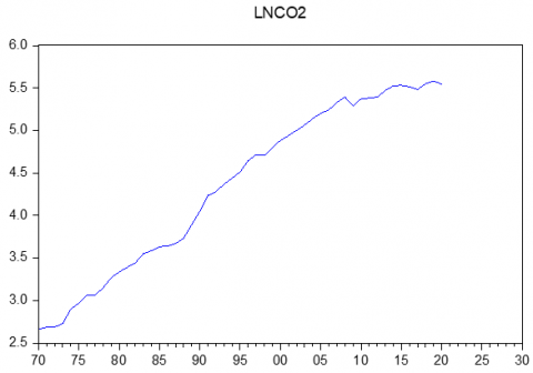
Figure 2. Smoothed series of the second-ordered difference series CO2 emission
However, since we are using the Automatic ARIMA Forecasting option in EViews for our forecasting purposes, the summary of the Automatic ARIMA Forecasting outcome directly provides the stationary level of the time series of LNCO2 emissions. According to the summary of Automatic ARIMA Forecasting outcomes as shown in Table 2, LNCO2 also stationary at the second-ordered differential. So, d=2. Adding to this, Figure 2 demonstrates that the second-ordered difference CO2 emission series values move toward upwards, which is consistent with the characteristics of a smooth series. Therefore, this indicates that the second-order differential carbon emission series is suitable for forecasting using the ARIMA model.
4.2 Determination of model parameters
Usually by observing the ACF and PACF correlogram plot, will determine the best order for p and q, and then use the resulting p, d, and q to develop an ARIMA model. There tend to be two conditions for the ACF and PACF of smoothed carbon emissions data in a model: Trailing or truncated. ACF or PACF functions are considered to have a truncated tail if their value is zero after lags p or q, respectively. If the lag order k raises, a trailing tail indicates that either the ACF or PACF function rot exponentially or oscillates to reach zero. Nevertheless, in the result of the Automatic ARIMA Forecasting summary, a model that meets the ARIMA models' tests is already present. According to the Automatic ARIMA Forecasting summary in Table 2, the ARIMA model (0, 2, 1) was the best choice because it fit the data the best for predicting CO2 emissions in Malaysia. Thereby, the p=AR (0), d=2, and q=MA (1).
4.3 Testing of the model
We have evaluated a thorough statistical analysis of the ARIMA model's results to assess its performance. Our analysis includes key goodness-of-fit measures such as R-squared (R2), Akaike Information Criterion (AIC), Schwarz Criterion, F-statistic, and likelihood of F-statistic. However, to have an effective model, SIGMASQ need to be small, Adjusted R-squared must be higher, AIC needs to be small, and there should be more significant coefficients [45, 46].
Table 3. ARIMA model (0,2,1) for Malaysia
|
Variable |
Coefficient |
Std. Error |
t-Statistic |
Prob. |
|
C |
-0.001138 |
0.001134 |
-1.003560 |
0.3208 |
|
MA (1) |
-0.882888 |
0.090837 |
-9.719510*** |
0.0000 |
|
SIGMASQ |
0.002719 |
0.000416 |
6.533004*** |
0.0000 |
|
R-squared |
0.382827 |
|||
|
Adjusted R-squared |
0.355994 |
|||
|
Akaike info criterion |
-2.916145 |
|||
|
Schwarz criterion |
-2.800319 |
|||
Note: ***, ** and * are significant at the 1%, 5% and 10% levels, respectively
As can be observed from Table 3, ARIMA (0,2,1) has lowest SIGMASQ, highest Adjusted R-squared, small AIC and the coefficient of MA is significant. the AIC and Schwarz Criterion results of -2.9161 and -2.8000, respectively, provide further insights into the model's fit. Adding to this, The R2 value of 0.3828 indicates that approximately 38.28% of the variance in the data is explained by the model. These measures collectively offer valuable insights into the effectiveness of the ARIMA model in capturing the underlying patterns in the CO2 emissions data.
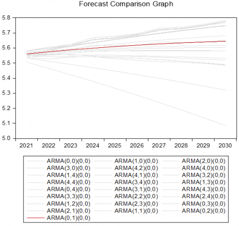
In the implementation of automatic ARIMA forecasting, forecast comparison graphs are an essential tool for assessing the accuracy of forecasting models. Figure 3 shows the some of the selected ARIMA model that relevant to the LNCO2 series. Based on Figure 3, the ARMA (0, 1) model is the best among all the models, represented by the red line in the graph.
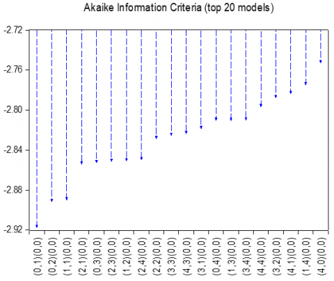
However, upon further examination of the Akaike Information Criteria (Top 20 Models) among all the models, the ARMA (0,1) model has the minimum AIC value (can refer Figure 4). It should be noted that the '0' refers to AR while the '1' refers to MA. The AIC value of the optimal model (ARIMA (0, 2, 1)) is -2.916145, which is relatively small compared to others, the fit accuracy is high. Therefore, the optimal model is ARIMA (0, 2, 1), and its specific equation is:
$\operatorname{LNCO2}_t=-0.001138-0.88288\,\, L N C O _2{t-1}+\varepsilon_t$
Figure 3. Forecast comparison graph
Figure 4. Akaike information criteria (Top 20 models)
4.4 Accuracy tests- ARIMA model
4.4.1 Diagnostic test 1: Correlogram Q statistics (correlogram of the residuals)
Utilizing the valid results acquired earlier, predictions are carried out employing the appropriate ARIMA model. The initial phase in this methodology involves confirming that the model meets the criteria for a stable univariate process. This verification entails ensuring that the residuals of the model exhibit white noise characteristics, as assessed through Ljung box Q statistics.
Null Hypothesis: Residuals are white noise.
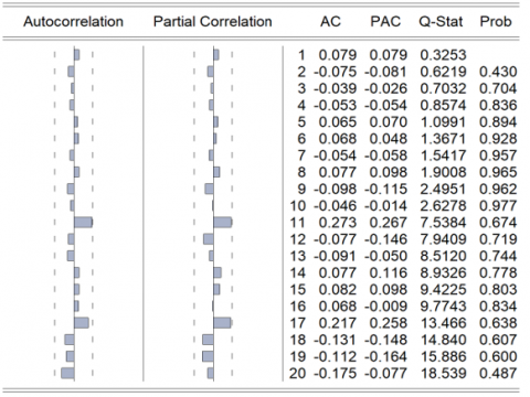
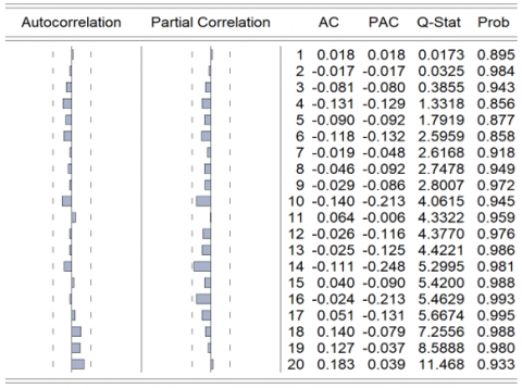
The graphs depicted in Figure 5 and Figure 6 reveal that there are no instances where values intersect the dotted lines for either autocorrelation or partial correlation. However, the p-values exceed 10 percent, implying that we are unable to reject the null hypothesis suggesting that the residuals conform to a white noise pattern.
Figure 5. Correlogram Q statistics
Figure 6. Correlogram of squared residual
4.4.2 Diagnostic test 2: ARMA process for (covariance) stationarity & invertibility
The second diagnostic examination involves assessing whether the estimated ARMA process is covariance stationary, a condition met when the AR roots fall within the unit circle. However, as our model has opted for AR (0), our focus will be solely on verifying invertibility.
To validate the invertibility of the estimated ARMA process, signifying that every MA root must be situated within the unit circle, we refer to Figure 7. The representation in Figure 7 confirms the invertibility of the ARMA process, as all data points are enclosed within the circle. With these criteria satisfied, we are now able to proceed with forecasting using the selected model.
Figure 7. ARMA structure
Further, following the ARIMA test, the relative residuals are minimal and the actual and fitted values of the data fitted well overall (as shown in Figure 8). Therefore, the model is generally valid and that the fit is good and the chosen ARIMA structure is stationary, and the model is accurately specified.
Figure 8. ARIMA (0, 2, 1) model test curve for the second-ordered difference series of the Malaysia CO2 emission
4.4.3 Diagnostic test 3: Heteroscedasticity
The ARCH test was employed to detect heteroscedasticity in the constructed model. The findings pertaining to the heteroscedasticity of residuals are presented in Table 4. The results indicate the absence of heteroscedasticity at a 5% significance level, as evidenced by a p-value of 0.899. This is attributed to the fact that the associated p-value associated with the F-statistic significantly exceeds the 5% significance level.
Table 4. Obtained results for checking heteroscedasticity of residuals
|
Heteroscedasticity: ARCH Test |
|||
|
F-statistic |
0.015435 |
Prob |
0.9017 |
|
Obs*R-squared |
0.016101 |
Prob |
0.8990 |
4.5 Forecasting analysing
Using the model of the ARIMA (0, 2, 1), we made static forecasts in-sample (1990–2020) to forecast 2021–2030 carbon emissions in Malaysia. The graphs in Figure 9 and Table 5 demonstrate our Malaysia’s forecasting results.
Figure 9. Actual and forecast value of CO2 emission of Malaysia
Table 5. Forecasted value of CO2 emissions (million tons) using the ARIMA (0, 2, 1) model
|
Year |
CO2 Emission (Million Tons) (In LN) |
CO2 Emission (Million Tons) (After Convert from LN) |
|
2021 |
5.5609 |
260.0576621 |
|
2022 |
5.5747 |
263.6818494 |
|
2023 |
5.5874 |
267.0523744 |
|
2024 |
5.5990 |
270.1582764 |
|
2025 |
5.6094 |
272.9893696 |
|
2026 |
5.6187 |
275.5362985 |
|
2027 |
5.6268 |
277.7905897 |
|
2028 |
5.6338 |
279.7446987 |
|
2029 |
5.6397 |
281.3920518 |
|
2030 |
5.6444 |
282.7270831 |
According to Philip et al. [46], Malaysia was one of the nations that committed to reducing its carbon emissions by 45 percent by 2030 at the 2015 United Nations Climate Change Conference. Therefore, this result could be valuable for stakeholders. The forecasting results below indicate that Malaysia's CO2 emissions are expected to continue rising in the coming years, albeit with a gradual decline. In our findings, the blue lines represent the predicted CO2 values, whereas the red lines represent the actual CO2 emissions. The finding indicates that the projected CO2 emissions for Malaysia are expected to rise annually, surpassing the threshold of approximately 5.6444 million tons/282.7270831 million tons by 2030 (refer Table 5) if Malaysia does not employ policies and mechanisms. Thus, this result fulfils the objective of the study we conducted.
The outcome is in line with previous studies by Tan et al. [32] showing that CO2 emissions have increased and are predicted to do so in the future particularly in Residential Buildings, Commercial and Public Services, and Transportation sectors. However, our findings were at contrast with those of Shekarchian et al. [31] and Kee et al. [34]. A key factor contributing to the disparities in our findings compared to previous studies could be the methodology used. To assess the impact on CO2 emissions levels, these articles utilized used renewable energy sources and Nonintrusive load monitoring (NILM)-based energy efficiency approaches in their study. This methodological variation likely influences the outcomes and may explain the divergence in findings. Besides, our use of ARIMA models, specifically the Box-Jenkins models, may introduce variations in the findings compared to studies utilizing different modelling techniques. Therefore, their findings differ from ours.
This points out that if Malaysia's CO2 emissions continue to increase in the future, which could be disastrous for the environment and puts a big question mark on Malaysia's policy of sustainability. If CO2 emissions continue to rise as predicted, the quality of the air will also degrade, which will eventually have an effect on human existence and other forms of life. However, the forecast amount of CO2 emissions is increasing at a slower pace. This could be a refer to the proper policy put in place to rising CO2 emissions with slower pace. The Malaysian authorities should therefore adopt the essential policy moves to address the growing issues of CO2 emissions.
In our forecasting model, we assumed that previous trends in CO2 emissions levels would persist into the future. While this assumption allowed us to leverage historical data to make predictions, it is essential to recognize its limitations. Future emissions levels may be influenced by many other factors that are not fully captured in the historical data. For instance, the introduction of carbon tax, new renewable energy policies or development in energy-efficient technologies could lead to significant shifts in emissions patterns. As such, even while our model provides insightful forecasts about possible future trends, it is essential to interpret the results with caution and consider the possible influence of external factors that may not have been accounted for in the model.
Greenhouse gases are the primary drivers of global climate change. CO2, as a significant component of greenhouse gases, plays a crucial role in environmental pollution and the phenomenon of global warming. The increase in global temperatures and the concentration of greenhouse gases in the atmosphere are causing significant changes in climatic conditions. It is extremely concerning since this climate change will have disastrous effects on crops, human well-being, the ecological balance, and biodiversity. A rise in CO2 dioxide emitted into the atmosphere is responsible for climatic changes and ecological imbalances. Malaysia classified as the highest CO2 emission contributor among the ASEAN countries. If we look at Malaysia's overall CO2 emissions, it rose by nine times, from 28 Mt in 1980 to 262.2 Mt in 2020. Therefore, recent years in Malaysia, urban and suburban populations have been hard hit by the disastrous effects of climate change brought on by the sharp increase in CO2 emissions, including floods, torrential downpours, heat waves, water shortages, and infrequent hailstorms. Thus, it is essential to analyse the detrimental impacts of humans and economy that contributes to the destructive effects towards environmental degradation in the form of CO2 emissions in Malaysia.
In addition to concerns about global warming and health issues brought on by Malaysia's poor air quality, this study looks into the impact of climate change, specifically focusing on the forecast of CO2 emissions. Therefore, this study aims to employ an ARIMA model for predicting CO2 emissions from 2021 to 2030. This study uses the Box-Jenkins model to apply automatic ARIMA forecasting within the EViews software in pursuit of robust and accurate forecasting. By leveraging the advanced capabilities of this methodology, we aim to provide an in-depth outlook on the trajectory of CO2 levels in Malaysia over the next decade. The Box-Jenkins model's application enables a thorough analysis of historical trends and the identification of key factors affecting carbon dioxide emissions due to its inherent adaptability to the nuances of time series data. The use of automatic ARIMA forecasting in EViews further enhances the precision and efficiency of our predictions. Upon preliminary analysis of the forecasted outcomes, an important discovery is revealed: during the following ten years, Malaysia's growing trend in carbon dioxide emissions is expected a gradual slowdown. Further the accuracy tests conducted on the ARIMA model provide compelling evidence of its robustness and effectiveness. This comprehensive accuracy assessment, including Correlogram Q Statistics, evaluation of the ARMA process, and analysis of relative residuals, collectively indicates that the ARIMA model performs well and provides a reliable representation of the underlying data dynamics.
Besides, this study contributes to knowledge by considering climate change policy in Malaysia. This study allowed government organizations and policymakers to discover the forecast value for 10 years, from 2021 to 2030, based on our findings. In light of Malaysia's pledge to the United Nations Framework Convention on Climate Change (UNFCCC) to accomplish a 45% reduction in CO2 emissions by 2030, this result may be useful. The recommendations provided in this study are intended for various stakeholders, including government authorities, financial institutions, private sectors, general public and international bodies. In light of Malaysia's goal to achieve net-zero greenhouse gas emissions by 2050, Malaysia's industrialization and income goals, the government should establish more stringent environmental regulations for industries. Both public and private sectors should invest in research centers to promote industrial waste as an energy source and reduce emissions. Considering the ongoing debate on carbon taxes, Malaysia should explore their implementation to foster sustainable growth. Notably, the Malaysian government has implemented the Green Technology Financing Scheme (GTFS) since 2010, aimed at promoting environmentally friendly practices. The GTFS provides financing options with an allocation of RM1.5 billion and offers a 2% interest subsidy to companies obtaining loans from participating banks for sustainable investments. It is recommended that Malaysia's central government should prioritize financial technology investments and develop financial regulations through monetary and fiscal policies to enhance the depth and efficiency of the country's financial system. Improving financial efficiency has the potential to reduce environmental risks while ensuring attractive returns on investments and savings.
The authors express sincere gratitude to all those who have made indirect contributions to the preparation of this manuscript.
[1] Merino-Saum, A., Baldi, M.G., Gunderson, I., Oberle, B. (2018). Articulating natural resources and sustainable development goals through green economy indicators: A systematic analysis. Resources, Conservation and Recycling, 139: 90-103. https://doi.org/10.1016/j.resconrec.2018.07.007
[2] Ling, C.H., Ahmed, K., Muhamad, R., Shahbaz, M., Loganathan, N. (2017). Testing the social cost of rapid economic development in Malaysia: The effect of trade on life expectancy. Social Indicators Research, 130: 1005-1023. https://doi.org/10.1007/s11205-015-1219-8
[3] Ahmed, Z., Wang, Z.H., Mahmood, F., Hafeez, M., Ali, N. (2019). Does globalization increase the ecological footprint? Empirical evidence from Malaysia. Environmental Science and Pollution Research, 26(18): 18565-18582. https://doi.org/10.1007/s11356-019-05224-9
[4] Global climate change. National Aeronautics and Space Administration (NASA). https://climate.nasa.gov/, accessed on Apr. 22, 2024.
[5] Global Energy Review 2020: The impacts of the Covid-19 crisis on global energy demand and CO2 emissions. 2021. International Energy Agency (EIA). https://www.iea.org/reports/global-energy-review-2020, accessed on Apr. 22, 2024.
[6] Chen, J.P., Huang, G., Baetz, B.W., Lin, Q.G., Dong, C., Cai, Y.P. (2018). Integrated inexact energy systems planning under climate change: A case study of Yukon Territory, Canada. Applied Energy, 229: 493-504. https://doi.org/10.1016/j.apenergy.2018.06.140
[7] Mei, H., Li, Y.P., Suo, C., Ma, Y., Lv, J. (2020). Analyzing the impact of climate change on energy-economy-carbon nexus system in China. Applied Energy, 262: 114568. https://doi.org/10.1016/j.apenergy.2020.114568
[8] Wang, L., Huang, G., Wang, X.Q., Zhu, H. (2018). Risk-based electric power system planning for climate change mitigation through multi-stage joint-probabilistic left-hand-side chance-constrained fractional programming: A Canadian case study. Renewable and Sustainable Energy Reviews, 82: 1056-1067. https://doi.org/10.1016/j.rser.2017.09.098
[9] Bozdağ, A., Dokuz, Y., Gökçek, Ö.B. (2020). Spatial prediction of PM10 concentration using machine learning algorithms in Ankara, Turkey. Environmental Pollution, 263(A): 114635. https://doi.org/10.1016/j.envpol.2020.114635
[10] Sarkar, M.S.K., Al-Amin, A.Q., Filho, W.L. (2019). Revisiting the social cost of carbon after INDC implementation in Malaysia: 2050. Environmental Science and Pollution Research, 26: 6000-6013. https://doi.org/10.1007/s11356-018-3947-1
[11] Karim, N., Othman, H., Zaini, Z.I.I., Rosli, Y., Wahab, M.I.A., Kanta, A.M.A., Omar, S., Sahani, M. (2022). Climate change and environmental education: Stance from science teachers. Sustainability, 14(24): 16618. https://doi.org/10.3390/su142416618
[12] Yaacob, M., So, W.W.M., Iizuka, N. (2022). Exploring community perceptions of climate change issues in peninsular Malaysia. Sustainability, 14(13): 7756. https://doi.org/10.3390/su14137756
[13] Begum, R.A., Raihan, A., Said, M.N.M. (2020). Dynamic impacts of economic growth and forested area on carbon dioxide emissions in Malaysia. Sustainability, 12(22): 9375. https://doi.org/10.3390/su12229375
[14] Malaysia | data and statistics. https://knoema.com/atlas/Malaysia, accessed on Feb. 23, 2022.
[15] Ehigiamusoe, K.U., Lean, H.H., Somasundram, S. (2022). Unveiling the non-linear impact of sectoral output on environmental pollution in Malaysia. Environmental Science and Pollution Research, 29: 7465-7488. https://doi.org/10.1007/s11356-021-16114-4
[16] Suki,N.M., Sharif, A., Afshan, S., Suki, N.M. (2020). Revisiting the environmental kuznets curve in Malaysia: The role of globalization in sustainable environment. Journal of Cleaner Production, 264: 121669. https://doi.org/10.1016/j.jclepro.2020.121669
[17] Khan, H.H., Samargandi, N., Ahmed, A. (2021). Economic development, energy consumption, and climate change: An empirical account from Malaysia. Natural Resources Forum, 45(4): 397-423. https://doi.org/10.1111/1477-8947.12239
[18] Zaman, N.A.F.K., Kanniah, K.D., Kaskaoutis, D.G. (2017). Estimating particulate matter using satellite based aerosol optical depth and meteorological variables in Malaysia. Atmospheric Research, 193: 142-162. https://doi.org/10.1016/j.atmosres.2017.04.019
[19] Tella, A., Balogun, A.L., Adebisi, N., Abdullah, S. (2021). Spatial assessment of PM10 hotspots using Random Forest, K-Nearest Neighbour and Naïve Bayes. Atmospheric Pollution Research, 12(10): 101202. https://doi.org/10.1016/j.apr.2021.101202
[20] World development indicators 2019. World Bank. https://datatopics.worldbank.org/world-development-indicators/, accessed on Feb. 23, 2022.
[21] Al-mulali, U., Solarin, S.A., Ozturk, I. (2019). Examining the asymmetric effects of stock markets on Malaysia’s air pollution: A nonlinear ARDL approach. Environmental Science and Pollution Research, 26: 34977-34982. https://doi.org/10.1007/s11356-019-06710-w
[22] Yuaningsih, L., Febrianti, R.A.M. (2021). The nexus between technological advancement and CO2 emissions in Malaysia. International Journal of Energy Economics and Policy, 11(6): 160-169. https://doi.org/10.32479/ijeep.11888
[23] Zhang, L.Y., Li, Z.C., Kirikkaleli, D., Adebayo, T.S., Adeshola, I., Akinsola, G.D. (2021). Modeling CO2 emissions in Malaysia: An application of maki cointegration and wavelet coherence tests. Environmental Science and Pollution Research, 28: 26030-26044. https://doi.org/10.1007/s11356-021-12430-x
[24] Alyousifi, Y., Ibrahim, K., Zin, W.Z.W., Rathnayake, U. (2022). Trend analysis and change point detection of air pollution index in Malaysia. International Journal of Environmental Science and Technology, 19: 7679-7700. https://doi.org/10.1007/s13762-021-03672-w
[25] Juneng, L., Latif, M.T., Tangang, F.T., Mansor, H. (2009). Spatio-temporal characteristics of PM10 concentration across Malaysia. Atmospheric Environment, 43(30): 4584-4594. https://doi.org/10.1016/j.atmosenv.2009.06.018
[26] World Bank. (2021). Economic Growth and Carbon Emission of Malaysia. https://data.worldbank.org/country/MY, accessed on Feb. 23, 2022.
[27] Adeel-Farooq, R.M., Raji, J.O., Qamri, G.M. (2023). Does financial development influence the overall natural environment? An environmental performance index (EPI) based insight from the ASEAN countries. Environment, Development and Sustainability, 25: 5123-5139. https://doi.org/10.1007/s10668-022-02258-x
[28] Aeknarajindawat, N., Suteerachai, B., Suksod, P. (2020). The impact of natural resources, renewable energy, economic growth on carbon dioxide emission in Malaysia. Environmental Science and Pollution Research, 10(3): 211-218. https://doi.org/10.32479/ijeep.9180
[29] Ehigiamusoe, K.U., Lean, H.H., Somasundram, S. (2023). Analysis of the environmental impacts of the agricultural, industrial, and financial sectors in Malaysia. Energy & Environment. https://doi.org/10.1177/0958305X231152480
[30] Sulaiman, A.S.M., Shabri, A., Marie, R.R. (2022) Forecasting carbon dioxide emission for Malaysia using fractional order multivariable grey model. Advances on Intelligent Informatics and Computing, 151-159. https://doi.org/10.1007/978-3-030-98741-1_14
[31] Shekarchian, M., Moghavvemi, M., Rismanchi, B., Mahlia, T.M.I., Olofsson, T. (2012). the cost benefit analysis and potential emission reduction evaluation of applying wall insulation for buildings in Malaysia. Renewable and Sustainable Energy Reviews, 16(7): 4708-4718. https://doi.org/10.1016/j.rser.2012.04.045
[32] Tan, C.H., Matjafri, M.Z., Lim, H.S. (2015). Prediction models for CO2 emission in Malaysia using best subsets regression and multi-linear regression. Remote Sensing of the Ocean, Sea Ice, Coastal Waters, and Large Water Regions, 9638: 963812. https://doi.org/10.1117/12.2195442
[33] Pauzi, H., Abdullah, L. (2014). Prediction on carbon dioxide emissions based on fuzzy rules. AIP Conference Proceedings, 1602(1): 222-226. https://doi.org/10.1063/1.4882491
[34] Kee, K.K., Lim, Y.S., Wong, J., Chua, K.H. (2021). Impact of nonintrusive load monitoring on CO2 emissions in Malaysia. Bulletin of Electrical Engineering and Informatics, 10(4): 1803-1810. https://doi.org/10.11591/EEI.V10I4.2979
[35] Malik, A., Hussain, E., Baig, S., Khokhar, M.F. (2020). Forecasting CO2 emissions from energy consumption in Pakistan under different scenarios: The China-Pakistan economic corridor. Greenhouse Gases: Science and Technology, 10(2): 380-389. https://doi.org/10.1002/ghg.1968
[36] Mustaffa, A.S., Shabri, A. (2020). An improved rolling NGBM (1,1) forecasting model with GRG nonlinear method of optimization for fossil carbon dioxide emissions in Malaysia and Singapore. In 2020 11th IEEE Control and System Graduate Research Colloquium (ICSGRC), Shah Alam, Malaysia, pp. 32-37. https://doi.org/10.1109/ICSGRC49013.2020.9232665
[37] Sulaiman, A.S.M., Shabri, A. (2021). Forecasting carbon dioxide emissions for Singapore using grey model with cramer’s rule. Malaysian Journal of Fundamental and Applied Sciences, 17(4): 437-445. https://doi.org/10.11113/MJFAS.V17N4.2091
[38] Ridzuan, A.R., Ismail, N.A., Hamat, A.F.C., Nor, A.H.S.M., Ahmed, E.M. (2017). Does equitable income distribution influence environmental quality? Evidence from developing countries of ASEAN-4. Pertanika Journal of Social Sciences and Humanities, 25(1): 385-400.
[39] The emissions database for global atmospheric research. European Union. EDGAR. https://edgar.jrc.ec.europa.eu/, accessed on May 9, 2024.
[40] Olivier, J.G.J., Bouwman, A.F., Maas, C.W.M.V.D., Berdowski, J.J.M. (1994). Emission database for global atmospheric research (Edgar). Environmental Monitoring and Assessment, 31: 93-106. https://doi.org/10.1007/BF00547184
[41] Box, G.E.P., Tiao, G.C. (1975). Intervention analysis with applications to economic and environmental problems. Journal of the American Statistical Association, 70(349): 70-79. https://doi.org/10.2307/2285379
[42] Alam, T., Alarjani, A. (2021). A comparative study of CO2 emission forecasting in the gulf countries using autoregressive integrated moving average, artificial neural network, and holt-winters exponential smoothing models. Advances in Meteorology, 2021: 8322590. https://doi.org/10.1155/2021/8322590
[43] Sen, P., Roy, M., Pal, P. (2016). Application of ARIMA for forecasting energy consumption and GHG emission: A case study of an Indian pig iron manufacturing organization. Energy, 116(1): 1031-1038. https://doi.org/10.1016/j.energy.2016.10.068
[44] Dickey, D.A., Fuller, W.A. (1979). Distribution of the estimators for autoregressive time series with a unit root. Journal of the American Statistical Association, 74(366): 427-431. https://doi.org/10.2307/2286348
[45] Kour, M. (2023). Modelling and forecasting of carbon-dioxide emissions in South Africa by using ARIMA model. International Journal of Environmental Science and Technology, 20: 11267-11274. https://doi.org/10.1007/s13762-022-04609-7
[46] Philip, L.D., Emir, F., Udemba, E.N. (2022). Investigating possibility of achieving sustainable development goals through renewable energy, technological innovation, and entrepreneur: A study of global best practice policies. Environmental Science and Pollution Research, 29: 60302-60313. https://doi.org/10.1007/s11356-022-20099-z