Alfina Taurida Alaydrus![]() | Adi Susilo
| Adi Susilo![]() | Agus Naba
| Agus Naba![]() | Suhayat Minardi*
| Suhayat Minardi*![]() | Anjar Pranggawan Azhari
| Anjar Pranggawan Azhari![]()
© 2024 The authors. This article is published by IIETA and is licensed under the CC BY 4.0 license (http://creativecommons.org/licenses/by/4.0/).
OPEN ACCESS
A comprehensive investigation has been conducted into the issue of seawater intrusion in the aquifer of the Mandalika Special Economic Zone (SEZ) on Lombok Island. Utilizing the RES2Dinv, Surfer13, and Rockwork software, data was processed in profiles and the time geoelectric resistivity survey method was implemented to monitor the velocity of seawater intrusion between 2021 and 2022. The findings of the study were segregated into three distinct transitional periods: a four-month transition from dry season to rainy season (Period I), a seven-month transition from dry season to intermediary conditions (Period II), and a year-long transition from dry season to dry season (Period III). The data revealed an expansion of the seawater intrusion zone from the south to the north at a depth range of 2 to 14 meters. This expansion was evidenced by a smaller volume of positive resistivity change in Period I compared to Period II. Moreover, a decrease in water content was observed in March 2022 measurements, leading to a less resistive, or more conductive, subsurface layer. In Period III, positive resistivity changes were solely identified in the western coastal area at a depth of 4 meters. Survey and measurement data indicated that seawater had infiltrated 12 coastal wells, with only wells 10 and 11 showing marginal mixing. This investigation underscores the escalating issue of seawater intrusion in the Mandalika SEZ aquifer, meriting urgent attention and mitigation strategies.
aquifer, electrical resistivity, conductivity, Mandalika, geochemistry
The Mandalika region, situated on the southern coast of Lombok Island, is under extensive development to bolster Indonesian tourism. Initially a coconut plantation and pond area, the landscape has undergone substantial transformation into a locale replete with hotels and other tourism-supporting accommodations. Such development necessitates an ample and quality water supply, leading to considerable and irregular exploitation of groundwater and coastal aquifers. These activities have resulted in the creation of void spaces within the aquifer, which subsequently become filled with seawater [1-5].
Seawater intrusion, a ubiquitous issue along global coastlines, significantly diminishes groundwater quality [6, 7]. This phenomenon, characterized by the movement of seawater inland and its replacement of freshwater, is dictated by fluid dynamics in coastal aquifers. The ensuing shift in the freshwater-seawater interface towards land is influenced by the disparity in density and pressure on either side of the interface [8]. Notably, excessive groundwater extraction activities in coastal regions can exacerbate seawater intrusion [1, 9], with implications not only for environmental integrity but also socio-economic development [10, 11].
To detect and monitor subsurface conditions based on their electrical properties, geophysical survey methods such as the resistivity geoelectric survey are frequently employed [11, 12]. The resistivity geoelectric method has been demonstrated to discern differences in resistivity contrast between freshwater and seawater [13]. Additionally, it has been used to track the movement of seawater in complex coastal aquifers by enabling repeated measurements over time, a technique known as time-lapse [1]. Although these studies have primarily focused on tracer tests with short monitoring periods [10], acknowledging seasonal variations necessitates a research approach that incorporates extended monitoring periods. This investigation aims to fill this research gap by implementing long-term monitoring and validating the geoelectric resistivity results with robust data.
Validation of the geoelectric resistivity survey can be achieved through groundwater quality measurements, which have indicated seawater mixing in some wells [14]. Geochemical analysis using groundwater quality standards—fresh water characterized by a conductivity value of <1200 μS/cm, a total dissolved solid (TDS) value of <0.50 gram/L, and a salinity value of <1000 ppt—can be applied for this purpose. Seawater intrusion leads to an increase in the TDS value, thereby significantly enhancing the conductivity value due to the high anion content originating from seawater contamination. This change is juxtaposed with a decrease in the resistivity value [15], which serves as an indicator of contamination; specifically, a low resistivity anomaly signifies seawater intrusion [1, 14].
The primary objective of this paper is to monitor seawater intrusion and ascertain the velocity of subsurface fluid movement in the Mandalika region. This is achieved by validating survey results through geochemical analysis of groundwater (TDS, salinity, and conductivity) as a technology for monitoring seawater intrusion, taking into account seasonal differences over a one-year period. It is assumed that only subsurface fluid movement occurred during this year, with the type of rock and its porosity remaining constant. This assumption is based on the understanding that physical changes in the subsurface structure cannot occur rapidly unless precipitated by extraordinary events such as earthquakes or tsunamis, meaning that changes in resistivity values are solely attributable to fluid dynamics/movements.
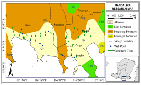
The study area is 10,000 km2, with a distance of 200 m from the coast line. The geological features in the study area are hills in the north and the Mandalika circuit in the south. The research locations covered four villages in the Mandalika area, including Kuta Village, Sukadana Village, Sengkol Village, and Mertak Village. The Mandalika area is on the subduction route of the Indo-Australian plate, which is in the coastal area in the southern part of Lombok Island and is directly adjacent to the Indian Ocean.
Figure 1. Geologic map of the study area
Geologically, the Mandalika SEZ area is a coastal area formed by alluvial processes. Alluvial plains are formed from sedimentary processes resulting from secondary deposition, so the rock compactness is relatively weak. As a result, pores are formed in the rock that allow intrusion to occur [3, 16, 17]. Figure 1 shows a map of the research location. It consists mainly of the Tomp Formation in the north and extends from Tanjung Aan to Merese Hill in the south. The Penggulung Formation is composed of tuff and breccia lava. Then in the south, it consists of alluvial layers and coastal deposits (Qa), the youngest rocks. Alluvial layers and coastal sediments are less compact rocks of sand, gravel, clay, and coral rubble. In addition, the southern region also has high permeability, so it has a considerable opportunity for seawater intrusion. Meanwhile, the Ekas Formation (Tme) is composed of limestone in the southeastern part. The Ekas Formation is located on Gerupuk Beach.
In this paper, the geoelectrical resistivity survey method is used over time to monitor the speed of seawater intrusion during specific periods between 2021-2022. This period is successively divided into three transitions: (i) period I start in August 2021 – December 2021 (dry to rainy season); (ii) period II starting in August 2021 – March 2022 (dry season to transition); (iii) period III starting from August 2021 – August 2022 (dry season to dry season). Two software RES2Dinv and Surfer13, are used to process data and present it in a 2D profile, while 3D profile data is processed using Rockwork software. Then the results of the geologic survey are validated based on the results of groundwater quality measurements, indicating that some of the wells have been mixed with seawater.
3.1 Geoelectrical resistivity
The measurement and collection of geoelectrical resistivity data used a G-sound geocis resistivity meter with 38 lines spread over the study area (Figure 1). The length of each resistivity geoelectric survey line is 120 m. Measurements were made above ground level with the help of current injection through two current electrodes (C1 and C2), then the potential difference was measured at the two potential electrodes (P1 and P2). According to study [16], the dipole-dipole configuration in resistivity geoelectric surveys is perfect for investigating shallow aquifers and lateral dispersion. Figure 2 shows the position of the dipole-dipole electrode configuration with a distance between the electrodes of 5 m, n (1-10). The dipole-dipole configuration involves current injection and potential measurement electrodes placed in a regular pattern. This pattern makes it possible to get a high-resolution picture of the resistivity variability around the aquifer [18, 19]. Because resistivity distribution is closely related to hydrogeological characteristics, it helps identify aquifer boundaries, sediment texture changes, and higher water potential zones.
Figure 2. The position of the electrodes in the Dipole-dipole configuration (Telford modification)
The output of the geoelectrical resistivity measurement method is expressed in apparent resistivity values. The apparent resistivity $\rho_a$ is defined as:
$\rho_a=\frac{\Delta V}{I} K_d$ (1)
where, $\rho_a=$ apparent resistivity $(\Omega \mathrm{m}), I=$ strong electric current (Ampere), $\Delta V=$ potential difference (Volts), $K_d=$ configuration geometry factor used where the dipole-dipole configuration factor is:
$K_d=\pi a(n)(n+1)(n+2)$ (2)
3.2 Time lapse geoelectrical
The resistivity geoelectric method over time is an implementation of the resistivity geoelectric method which is executed at the same point at different times. The application of the resistivity geoelectric method over time was carried out with four measurements as shown in Table 1. The change in the apparent resistivity value over time at the same point is calculated using Eq. (3).
Table 1. Data collection timeline
|
Measurement Number |
Time |
Rainfall |
Season |
|
1 |
August 2021 |
<20 mm |
Dry |
|
2 |
December 2021 |
301-400 mm |
Rain |
|
3 |
March 2022 |
151-200 mm |
Transition |
|
4 |
August 2022 |
<20 mm |
Dry |
$\Delta \rho=\rho_{n+1}-\rho_n$ (3)
where, ∆ρ is the change in true resistivity over time (Ωm), ρ is the true resistivity value at the time (Ωm) and, n is measurement time number (1, 2, 3, and 4).
Furthermore, the velocity of fluid movement is calculated by comparing the volume of changes over time based on 3D modeling with Eq. (4).
Fluid speed $=\frac{\text { Change volume }}{\text { Time lapse }}$ (4)
where, speed of fluid movement in m3/month, the volume of fluid change over time in m3 and, time interval in months. The analysis was carried out by reviewing and interpreting changes in the apparent resistivity values and the velocity of fluid movement in measurements between 2-1, 3-1, and 4-1.
3.3 Analysis of groundwater samples
Geochemical data were obtained by measuring samples of 12 groundwater wells near the geoelectrical track (Figure 1) to correlate the parameter analysis. The physical parameters measured in groundwater samples were conductivity, TDS, and salinity using the EC meter (Electrical Conductance) model 9000. Geochemical data measurements for groundwater quality were repeated four times from August 2021 to August 2022, with details in Table 1.
4.1 2D profile of geoelectrical resistivity
Processing of 2D geoelectrical resistivity data results was carried out on 38 resistivity sections for each measurement period. However, only four resistivity sections are interpreted as representing measurement sections that are close together and have a similar pattern, including: Line 2, Line 17, Line 23, and Line 36. In general, subsurface resistivity cross-sections illustrate the contrast of low resistivity values and resistivity values. ground water level. Groundwater electrical resistivity values vary from 10 to 100 Ωm depending on the TDS concentration [20]. The value of the electrical resistivity of groundwater changes to become smaller if the chemical content is greater. Table 2 shows the resistivity value levels and zone indications obtained from several previous researchers.
Table 2. Distribution of resistivity levels and their indications
|
No. |
Levels |
Resistivity Value (Ωm) |
Contour Colour |
Zone Indication |
Ref. |
|
1. |
Low |
<10 |
Purple-Green |
saline zone or seawater intrusion |
[11, 14, 21] |
|
2. |
Middle |
10-50 |
Light green-orange |
transition zone or brackish water zone |
[14] |
|
3. |
High |
50-100 |
Dark orange-red |
freshwater zone in general |
[14, 20] |
Based on Figures 3-6, it can be seen that a high resistivity value indicates the freshwater zone. The high resistivity value decreases gradually, indicating a seawater intrusion zone. The front boundary between fresh water and seawater is at a depth of 8 meters, and most do not have clear boundaries. The location of the boundary between freshwater and seawater changes depending on seasonal conditions. During the rainy season, the boundary between fresh water and seawater widens. However, the resistivity value becomes more significant, indicating that the zone is a dispersion zone or a zone of mixing fresh water with seawater.
Figure 3. The 2D geoelectric resistivity profile of Line 2: (a) 1st measurement; (b) 2nd measurement; (c) 3rd measurement; (d) 4th measurement
Figure 3 shows the subsurface cross-section of the 1st to 4th resistivity geoelectric survey results. As seen in Figures 3(a) and 3(d), the subsurface section of line 2, which is in the west and near the Kuta Mandalika coastline, has a resistivity range between 1.2 – 1022.9 Ωm. Figure 3(a) shows the color contours, dominated by orange and red, which show medium to high resistivity values. That indicates a layer of rock that contains fresh water. On the other hand, the purple to green colors shows slight to moderate values spread at a depth of 3-9 meters below the surface, indicating seawater intrusion into the mainland. In the second measurement (Figure 3(b)), it can be seen that the color contours are dominated by green and yellow, indicating moderate resistivity values. That indicates that the rock layer contains fresh water, and the resistivity value has decreased. That is because the measurements were taken during the rainy season, so the rock layers are more conductive, causing the resistivity value to be smaller. The purple to blue colors, which show small resistivity values, is spread at a depth of 3 - 9 meters below the surface, indicating seawater intrusion.
Furthermore, in the third measurement (Figure 3(c)), the color contour is dominated by purple to blue. Seawater intrusion indicates a small resistivity value 6 -10 meters below the surface. The distribution of purple to blue colors at this depth is increasingly widespread, which indicates a broader intrusion of seawater. On the other hand, the fourth measurement (Figure 3(d)) was carried out during the dry season; the color contour was dominated by orange to red, indicating a moderate to high resistivity value, the same as the first measurement. It can be seen that the resistivity value increased in the fourth measurement compared to the second and third measurements. That is because the measurements were carried out during the dry season, which caused the rock layers to tend to be more resistive. Hence, the resistivity values of the rock layers in the measurement area became more significant. In addition, the distribution of purple to blue contours is still scattered at a depth of 6-9 m below the surface, which indicates seawater intrusion at that depth.
Figure 4. Geoelectric resistivity 2D cross-sectional profile of Line 17: (a) 1st measurement; (b) 2nd measurement; (c) 3rd measurement; (d) 4th measurement
Figure 4 shows a subsurface cross-section of line 17 in the northern part of the Mandalika circuit. In line 2, intrusion can occur at a depth of about 3 to 9 m below the surface, which is indicated by purple to blue colors, which show small resistivity values evenly distributed at that depth. Figure 4(a) shows that the distribution of purple to blue colors is located at a depth of 3 – 9 meters below the surface, which indicates an intrusion at that depth. Then underneath, there is a red color indicating a rock with a higher resistivity and a layer of fresh rock. Meanwhile, Figure 4(b) shows that the distribution of purple to blue colors is getting bigger or wider because the measurements were taken to coincide with the rainy season, causing the resistivity around the measurement area to tend to decrease in value. However, it can be seen that the position of the purple and blue distribution is still at a depth of around 3 to 9 m which indicates intrusion occurred at that depth.
Furthermore, Figure 4(c) shows that the distribution of purple to blue does not change significantly. It has almost the same pattern indicating no significant change in intrusion conditions from the second measurement. Then Figure 4(d) has a similar contour as Figure 4(a) because the measurements were carried out in the same season (dry season). Thus, the rock layers around the measurement area become more resistive so that the resistivity value increases, marked by a distribution of yellow to orange colors. The distribution of blue-orange purple is found at a depth of about 3 – 9 meters below the surface which is indicated where there is an intrusion.
Figure 5. Geoelectric resistivity 2D cross-sectional profile of Line 23: (a) 1st measurement; (b) 2nd measurement; (c) 3rd measurement; (d) 4th measurement
Figure 5 shows the subsurface cross-section of line 23 on the south coast of Tanjung Aan Beach and has a resistivity range between 0.5 – 345.1 Ωm. The subsurface section of line 23 is dominated by a water-saturated layer intruded by seawater. The thickness of the seawater intrusion zone on line 23 ranges from 6 meters in the north and 3 – 12 meters in the south. As shown in Figure 5(a), the purple-to-blue color distribution is located 3 – 9 meters below the surface. That indicates an intrusion at that depth, and below it, a red color indicates a rock with a higher resistivity which indicates a layer of fresh rock. On the other hand, in Figure 5(b), there is a more significant or broader distribution of purple to blue colors because the measurements were taken to coincide with the rainy season, causing the resistivity around the measurement area to decrease in value. However, it can be seen that the position of the distribution of purple and blue colors is still at a depth of around 3 to 9 m, which indicates intrusion occurred at that depth.
Furthermore, Figure 5(c) shows a distribution of purple to blue colors that do not change significantly, like Figure 5(b). However, it has almost the same pattern, indicating no significant change in intrusion conditions from the second measurement. Meanwhile, Figure 5(d) has a similar contour as the first measurement (Figure 5(a)). That is because the measurements were taken in the same season. In the dry season, the rock layers around the measurement area become more resistive so that the resistivity value increases, marked with a distribution of yellow to orange colors. The distribution of blue-orange purple is found at a depth of about 3-9 meters below the surface where there is an intrusion. The dynamics of changes in the seawater intrusion zone again occur in the dry season of the fourth measurement (Figure 5(d)), where purple, green, to orange contours are found almost along the track, which indicates that seawater intrusion is getting more massive over time when compared to the first measurement with the same season.
Figure 6. Geoelectric resistivity 2D cross-sectional profile of Line 36: (a) 1st measurement; (b) 2nd measurement; (c) 3rd measurement; (d) 4th measurement
This cross-section of line 36 has the smallest resistivity value among the resistivity values of all lines, as shown in Figure 6. The thickness of the seawater intrusion zone on line 36 ranges from 5-6 meters along the track. The subsurface section of line 36, which is in the eastern part of the Mertak area, has a resistivity range between 0.4 – 222.6 Ωm. Figure 6(a) shows the distribution of purple to blue colors located at a depth of 3 – 9 meters below the surface, indicating an intrusion at that depth. Then at the bottom, there is an orange color indicating a rock with a higher resistivity and a layer of fresh rock. Figure 6(b) is the second measurement made in December 2021; the distribution of purple to blue colors is getting bigger or broader in the surface area. That is because the measurements were taken to coincide with the rainy season, causing the resistivity around the measurement area to tend to decrease in value. However, at a depth of about 3 to 9 m, it shows the position of the distribution of purple and blue colors, indicating that intrusion occurred at that depth.
Similar to Figures 4(c) and 5(c), Figure 6(c) also has a purple-to-blue distribution, which has not changed significantly from the second measurement (Figure 6(b)). It has almost the same pattern, indicating no significant change in intrusion conditions from the second measurement. Likewise, with Figure 6(d), the measurements were carried out in August 2022, or the dry season. It has the exact contour resemblance as the first measurement (Figure 6(a)). Because the measurements were carried out during the dry season, the rock layers around the measurement area became more resistive. Hence, the resistivity value increased, marked by a distribution of yellow to orange colors. The distribution of blue-orange purple is found at a depth of about 3 – 9 meters below the surface where there is an intrusion.
4.2 Geoelectrical resistivity time lapse
4.2.1 Period I (August 2021 – December 2021)
Period I is the phase from the dry to the rainy season, lasting four months. Geoelectrical resistivity measurements time lapse is carried out to monitor processes and dynamics of specific parameters based on changes in subsurface resistivity, such as monitoring seawater intrusion in coastal areas [11, 22]. Subsurface resistivity changes are obtained by determining the difference in resistivity values between the two periods at the same point. The change value is entered with RES2DINV to produce the resistivity distribution, as shown in Figure 7.
Figure 7. Differences in resistivity values in the August 2021 and December 2022 periods: (a) Line 2; (b) Line 17; (c) Line 23; (d) Line 36
Changes in resistivity values are categorized into three categories: positive changes, negative changes, and unchanged or constant. A positive change means that the resistivity value in the final measurement is greater than the resistivity value in the initial measurement. That is possible because sea water is replaced by fresh water. Conversely, a negative change means that the resistivity value at the end of the measurement is smaller than the resistivity value at the initial measurement. These negative changes indicate a widening/expansion of seawater intrusion. That is possible if fresh water in the study area is replaced by seawater intrusion that occurs. An unfavorable change means that the resistivity value in the final measurement is smaller than the resistivity value in the initial measurement. These negative changes indicate a widening or expansion of seawater intrusion.
Negative resistivity change means that the resistivity value of the final measurement is smaller than the resistivity value of the initial measurement. That is possible if fresh water in the study area is replaced by seawater intrusion occurs. Vice versa, a positive change in resistivity means that the resistivity value of the final measurement is greater than the initial measurement's resistivity value, which is possible because seawater is replaced by fresh water.
As shown in Figure 7(a), the geoelectrical resistivity over time at line 2 in the north indicates that the zone is contaminated with seawater. At a depth of 2 – 9 meters, this zone experiences a positive value change, indicating an increase in the electrical resistivity value. Then in the dry season, the resistivity value of the intrusion zone or contaminated with sea water is <4 Ωm, and this zone increases during the rainy season to <7 Ωm. This increase is directly related to a decrease in the level of contamination or salinity of groundwater in the zone due to rainwater infiltration into the aquifer. However, in contrast to the southern part of line 2, adverse changes are predominant in most sections due to seawater infiltration from the coast. According to study [7], changes in the electrical resistivity values in Figure 8(a) are very likely to occur, considering that the aquifers in this zone are free aquifers where the layers overlap with alluvium and sandstone.
Furthermore, Figure 7(b) shows the resistivity distribution over time at line 17. This zone is contaminated with seawater on the left at a depth of 9 m, which changes in positive resistivity values. In the dry season, the resistivity value of the intrusion zone or contaminated seawater in the north and south is smaller than in the rainy season. Changes in value only ranged from < 5 Ωm to < 9 Ωm. Like line 2, zone 17 also experiences rainwater infiltration into the aquifer. However, the intrusion zone (<10 Ωm) on the right is more comprehensive to the north and thicker during the rainy season than the intrusion zone in the dry season, accompanied by a decrease in the electrical resistivity value (Figure 4(b)).
Meanwhile, Figure 3(c-d) and Figure 4(c-d) show changes in the zoning at line 23 and line 36. There is an apparent change that the seawater intrusion zone that appears during the dry season extends northward, accompanied by a decrease in resistivity values during the rainy season (Figure 7(c-d)). This change in the seawater intrusion zone is similar to the change in the intrusion zone on line 2 but different from the widening of the intrusion zone on line 17. Likewise, line 23 is very close to the Tanjung Aan shoreline, and line 36 on the east coast of Mertak Village allows infiltration of seawater onto land to be easier if there is a vacancy of fresh water.
Based on the modeling results for the period August 2021 to December 2022, as shown in Figure 8(a), it is shown that the change in resistivity values ranges from -1,841.85 - 677.86 Ωm. In the southwest, with a depth of 4 – 14 m, there is a change in the negative zone, which is more comprehensive, and the difference in value gets more significant with increasing depth. The negative change zone expands as the depth increases, meaning that the negative zone expands with increasing depth, indicating that the seawater zone is more expansive laterally below the surface. That is following several studies which state that fresh water seems to be floating above sea water because fresh water is immiscible with sea water under seawater intrusion in free aquifers. The negative zone that appears near the surface of Kuta Mandalika is probably caused by a decrease in the freshwater level in the study area followed by an increase in the seawater interface [1, 23]. This decrease is indicated by the excessive pumping/collecting of fresh water at that location [24].
Figure 8. 3D pseudosection of changes in resistivity values from August to December 2021: (a) Total; (b) Constant; (c) Positive; (d) Negative
In contrast, positive changes appear in the southeastern part from the surface to a depth of 2 m and in the northeast from a depth of 4-14 m. Assuming the uncertainty of the measurement results is 5%, the change in resistivity values in the range of -92.09 to 33.89 Ωm is considered unchanged or constant. In other words, a change in resistivity value >33.89 Ωm is a positive change, and a change in resistivity value <92.09 Ωm is a negative change. The zone of change in resistivity values during the measurement period is shown in Figure 8(b-d). The fluid volume that experienced positive changes, negative changes, and constant was 8,300,000 m3 (2.47%), 101,460,000 m3 (30.20%), and 226,240,000 m3 (67.33%), respectively. The volume of change in the negative resistivity value, which is greater than the volume of positive change, is thought to be due to water infiltration from the surface in the rainy season, so the conductivity value increases. The volume of fluid movement from August 2021 to December 2021 is 109,760,000 m3 with a speed of 27,740,000 m3/month.
4.2.2 Period II (August 2021 – March 2022)
Period II is the dry season phase to the transition season, which lasts for seven months. The results of modeling the change in apparent 3D resistivity values from August 2021 to March 2022 are shown in Figure 9(a).
Figure 9. Pseudosection 3D change in resistivity values August 2021 to March 2022: (a) Total; (b) Constant; (c) Positive; (d) Negative
Changes in resistivity values in this period ranged from -1986.94 to 1548.62 Ωm. At a 2 – 14 m depth, the western part is dominated by a negative change zone. This negative change zone expands with increasing depth, with the most significant negative change value range being at a depth of 10 – 12 m (dark blue level). Likewise, in the southeastern part, there is a zone of negative change on the surface to a depth of 2 m, followed by a zone of positive change from a depth of 2–14 meters. Assuming the uncertainty of the measurement results is the same, the positive change zone volume is 20,380,000 m3 (6.07%), the negative change zone volume is 76,180,000 m3 (22.68%), and the constant zone volume is 239,400,000 m3 (71.25%) (Figure 9(b-d)). The volume of change in the negative resistivity value, which is greater than the volume of positive change, is thought to be due to water infiltration from the surface during the rainy and transitional seasons, so the conductivity value increases. The volume of fluid movement from August 2021 to March 2022 is 96,560,000 m3 with a speed of 13,794,285 m3/month.
4.2.3 Period III (August 2021 – August 2022)
Figure 10. The 3D pseudo section of changes in resistivity values in the period August 2021 to August 2022: (a) Total; (b) Constant; (c) Positive; (d) Negative
This measurement period lasts 12 months with the dry season phase to the next dry season. Figure 10(a) shows a pseudo-3D model of changes in period III resistivity values ranging from -832 Ωm to 4,168 Ωm.
The negative change zone pattern is similar to the period I change a pattern, but the positive change zone pattern is different. The zone of positive change in these 12 months is shown in Figure 10(c), which has a thickness of 2 meters from the surface and dominates the western part of the study area. The volume of the zone of positive change, negative change, and constant in the 12 months, respectively, is 8,180,000 m3 (2.44%), 103,140,000 m3 (30.70%), and 224,660,000 m3 (66.86%). The volume of fluid movement from August 2021 to August 2022 is 111,320,000 m3 with a speed of 9,276,666 m3/month.
Table 3. Groundwater sample quality data in the Mandalika area
|
Sample |
Salinity (ppt) |
TDS (grams/L) |
Conductivity (µS/cm) |
|||||||||
|
Measurement to- |
Measurement to- |
Measurement to- |
||||||||||
|
1 |
2 |
3 |
4 |
1 |
2 |
3 |
4 |
1 |
2 |
3 |
4 |
|
|
Well 1 |
0.95 |
0.91 |
0.76 |
0.79 |
1.18 |
1.33 |
1.1 |
1.15 |
1644 |
1770 |
1596 |
1644 |
|
Well 2 |
2.17 |
2.1 |
1.77 |
2.91 |
3.07 |
3.11 |
2.66 |
4.34 |
3700 |
4060 |
3530 |
5140 |
|
Well 3 |
1.04 |
0.46 |
0.47 |
1.03 |
1.34 |
0.65 |
0.66 |
1.37 |
1869 |
919 |
961 |
1542 |
|
Well 4 |
1.24 |
0.3 |
0.61 |
0.86 |
1.62 |
0.42 |
0.88 |
1.23 |
2250 |
603 |
1284 |
1868 |
|
Well 5 |
1.01 |
0.81 |
0.89 |
0.79 |
1.33 |
1.23 |
1.31 |
1.14 |
1850 |
1663 |
1852 |
1628 |
|
Well 6 |
0.9 |
0.5 |
0.39 |
0.56 |
1.2 |
0.71 |
0.55 |
0.8 |
1663 |
1020 |
824 |
1161 |
|
Well 7 |
1.31 |
2.65 |
0.88 |
2.3 |
1.77 |
3.93 |
1.29 |
3.44 |
2430 |
4970 |
1822 |
4580 |
|
Well 8 |
4.15 |
0.38 |
0.93 |
1.05 |
5.47 |
0.55 |
1.37 |
1.54 |
7340 |
778 |
1920 |
2130 |
|
Well 9 |
1.4 |
1.1 |
0.97 |
0.97 |
1.88 |
1.59 |
1.42 |
1.41 |
2590 |
2150 |
1997 |
1971 |
|
Well 10 |
0.7 |
0.65 |
0.57 |
0.53 |
0.92 |
0.94 |
0.82 |
0.76 |
1295 |
1288 |
1193 |
1109 |
|
Well 11 |
0.5 |
0.42 |
0.46 |
0.41 |
0.67 |
0.59 |
0.65 |
0.58 |
944 |
860 |
959 |
847 |
|
Well 12 |
1.18 |
1.08 |
0.97 |
1.04 |
1.6 |
1.57 |
1.41 |
1.53 |
2210 |
2140 |
1981 |
2110 |
4.3 Geochemistry of groundwater samples
Table 3 compares geochemical parameters of groundwater quality over time in 12 wells. As seen in the table, it can be stated that most of the fresh water in the study area has been mixed with seawater except for wells 10 and 11 which are still slightly mixed with seawater. This indication is based on the TDS test conducted in the dry season 2 times. The first and fourth tests obtained TDS 0.92 and 0.76 in healthy 10, while well 11 obtained TDS 0.67 and 0.58. This determination is based on groundwater quality standards which are declared fresh water if the conductivity value is <1200 µS/cm, the TDS value is <0.50 gram/L [20], and the salinity value is <1000 ppt. Groundwater quality values at the study sites varied according to the season, where the values of salinity, TDS, and conductivity tended to be higher in the dry season than in the rainy season.
4.4 Discussion
Seawater intrusion is a global environmental phenomenon affecting the chemical composition of coastal groundwater, and this may become more critical shortly due to increasing sea level rise associated with a changing climate [25]. Moreover, growing water demand and manipulation of natural hydrological systems have led to saltwater intrusion being considered a significant future threat to coastal freshwater resources globally [26-28]. In this paper, the thickening and expansion of intrusion areas are caused by seasonal changes, measurement periods, and water use (pumping) in the Mandalika coastal area. That can be proven based on the investigation results, namely that all trajectories have the same pattern and at the same average depth between 3 – 9 meters below the surface. These results have also been validated through biochemical tests with salinity, TDS, and conductivity indicators. The four tests with different seasons show freshwater have experienced mixing with sea water indicated by TDS, salinity, and higher conductivity values than typical values. According to study [29], mixing seawater and fresh water in seawater intrusion makes fresh water increasingly saline because the total dissolved solid content increases. Furthermore, in the future, efforts to understand the processes and causes of seawater intrusion holistically can be carried out by taking into account various natural factors such as sea level changes, weather and climate changes, coastal erosion, and subsidence of the surface land, as well as human-caused factors such as groundwater extraction/pumping rate.
The results of the 2D resistivity inversion show that the electrical resistivity value of the Mandalika beach area ranges from 0.4 - 1,022.9 Ωm with different fluid contents. The electrical resistivity of the Mandalika beach area is dominated by low electrical resistivity <10 Ωm with indications of seawater intrusion into the surrounding aquifers. The dominant low resistivity is in the western part of Kuta Mandalika Beach at a depth of 2 to 11 meters and in the eastern part around Tanjung Aan Beach and Mertak Village at 3-12 meters. The results of this study state that seawater has infiltrated the coastal aquifer in the Mandalika area. According to study [30], the geoelectrical survey method can predict the distribution pattern of subsurface resistivity values by measuring the ground surface. Geophysics can describe stratigraphic units and shows that the salt zone decreases as one moves away from the coast. Subsurface resistivity is also related to geological parameters such as mineral content, porosity, and the level of water saturation in rocks and soil [31]. Another method that can be used to determine indications of seawater intrusion is to use resistivity imaging to evaluate geoelectrical parameters as has been done by other researchers on the East coast of Virginia [32], Abu Zenima, West Sinai-Egypt [29], and Digha-East India [29, 30]. In addition, several other works also illustrate that the resistivity method is a fast and efficient method for mapping interfaces in an area [31-33].
Table 4. Summary of subsurface fluid dynamics from August 2021 to August 2022
|
Period |
Duration (month) |
Fluid Dynamics (m3) |
Speed (m3/month) |
||
|
Positive |
Negative |
Constant |
|||
|
08/21 – 12/21 |
4 |
8.300.000 |
101.460.000 |
226.240.000 |
27.740.000 |
|
08/21 – 03/22 |
7 |
20.380.000 |
76.180.000 |
239.400.000 |
13.794.285 |
|
08/21 – 08/22 |
12 |
8.180.000 |
103.140.000 |
224.660.000 |
9.276.666 |
Another finding in this paper is the subsurface fluid dynamics movement pattern for one year, as shown in Table 4. Intrusion occurs because the position of fresh water is replaced by seawater; this is possible if the excessive and continuous withdrawal of fresh water is carried out, disrupting the groundwater balance. That happens along with seasons and land use changes where many hotels and settlements are built. The results of this study can be helpful to the government as a reference in the exploitation and exploration of groundwater and in maintaining environmental balance in the Mandalika area.
The volume of constant resistivity in the three periods in Table 4 is relatively the same, while the volume of positive and negative resistivity changes varies. The volume of change in positive resistivity during the dry season to the rainy season is smaller than that from the dry season to the transitional season. That indicates that the water content contained at the time of measurement of rainfall is decreasing so that the subsurface layer becomes less resistive or more conductive. Factors causing this include reduced groundwater extraction and natural recharge water that enters the subsurface. However, for one year (August 2021-August 2022), positive resistivity changes only appear in the western part of the Kuta Mandalika Beach area, which reaches a depth of 4 meters. The suspected cause of the positive resistivity change on the Kuta Mandalika beach is over-pumping to meet the needs of the high population and support tourism activities [34, 35] since early 2022, which has been increasing rapidly. Over pumping is characterized by a decrease in the groundwater level up to 2.6 meters.
Furthermore, the volume of adverse changes in the dry season to the rainy season is more significant than in the rainy season to the transition period. That is because, in December 2021, rainfall in the study area was very high (range 301 – 400 mm), while in March 2022, rainfall was classified as moderate (range 151 – 200 mm). During the rainy season, rainwater infiltrates below the surface, which makes rocks that were initially dry contain more and more water so that rocks become more conductive or less resistive [10, 36].
From August 2021 to August 2022, the volume of negative changes is the highest. Supposedly the volume of adverse changes in the dry season decreases due to water loss. However, in August 2022, the volume of negative changes increased. That is caused by the disturbance of the groundwater-seawater balance in the aquifer, so the seawater contamination zone is increasing in the eastern part (the coast of Tanjung Aan). Indications of increased contamination by seawater intrusion are further strengthened by wells 2 and 3, which are close to the coast of Tanjung Aan and have high salinity values ranging from 2.91 - 3.0 ppt (Figure 3(a)), high TDS values ranging from 4.34 - 13.7 g/liter (Figure 3(b)), and high conductivity ranging from 1542 – 5140 μS (Figure 3(c)) during the August 2022 dry season. In addition, the groundwater level in the well has increased from 2.05 m to 3.0 – 3.06 meters. The increase in contamination levels and the expansion of the seawater contamination zone in the east of the study area are significantly influenced by the tides in the Indian Ocean [1, 37]. Spatial differences in sea level rise due to climate change or rainfall [38] affect the groundwater level, especially during the dry season [39].
The Mandalika SEZ has generally experienced seawater intrusion, characterized by electrical resistivity ranging from 0.4 – 1022.9 Ωm with different fluid content differences. In comparison, electrical resistivity is dominated by low electrical resistivity <10 Ωm. This condition is dominant in the western part of Kuta Mandalika Beach at a depth of 2 meters to 11 meters and in the eastern part around Tanjung Aan Beach and Mertak Village at 3-12 meters.
The dynamics of subsurface fluid movement, calculated based on 3D visualization of changes in resistivity values, shows positive, adverse, and constant change zones. The calculation results show that the speed of fluid movement from August 2021 to August 2022 is getting slower. Changes in electrical resistivity values and groundwater quality parameter values in the study area have changed over time, becoming increasingly saline due to seasonal differences and human-caused factors such as over-exploitation of groundwater.
The authors would like to thank the Ministry of Education, Culture, Research and Technology, Republic of Indonesia for the supported research funding with Certificate number 108/E4.1/AK.04.PT/2021.
|
SEZ |
Special Economic Zone (SEZ) |
|
TDS |
Total Dissolved Solid |
|
Qa |
Coastal deposits |
|
Tme |
Ekas Formation |
|
Greek symbols |
|
|
ρa |
Apparent resistivity, Ωm |
|
∆ρ |
Change in true resistivity over time, Ωm |
|
ρ1 |
The true resistivity value at the 1st time, Ωm. |
|
ρ2 |
The true resistivity value at the 2nd time, Ωm |
|
I |
Strong electric current, Ampere |
|
∆V |
Potential difference, Volts |
|
Kd |
Configuration geometry factor |
[1] McDonnell, M.C., Flynn, R., Águila, J.F., Hamill, G.A., Donohue, S., Benner, E.M., et al. (2023). Four-dimensional electrical resistivity imaging for monitoring pumping-induced saltwater intrusion in a coastal aquifer. Science of the Total Environment, 867: 161442. https://doi.org/10.1016/j.scitotenv.2023.161442
[2] Bhattacharjya, R.K., Datta, B., Satish, M.G. (2009). Performance of an artificial neural network model for simulating saltwater intrusion process in coastal aquifers when training with noisy data. KSCE Journal of Civil Engineering, 13: 205-215. https://doi.org/10.1007/s12205-009-0205-6
[3] Prusty, P., Farooq, S.H. (2020). Seawater intrusion in the coastal aquifers of India-A review. HydroResearch, 3: 61-74. https://doi.org/10.1016/j.hydres.2020.06.001
[4] Barlow, P.M. (2003). Ground water in freshwater-saltwater environments of the Atlantic Coast. US Department of the Interior, US Geological Survey.
[5] Giordano, R., Milella, P., Portoghese, I., Vurro, M., Apollonio, C., D'Agostino, D., Lamaddalena, N., Scardigno, A., Piccinni, A.F. (2010). An innovative monitoring system for sustainable management of groundwater resources: Objectives, stakeholder acceptability and implementation strategy. In 2010 IEEE Workshop on Environmental Energy and Structural Monitoring Systems, Taranto, Italy, pp. 32-37. https://doi.org/10.1109/EESMS.2010.5634172
[6] Alhumimidi, M.S. (2020). An integrated approach for identification of seawater intrusion in coastal region: A case study of northwestern Saudi Arabia. Journal of King Saud University-Science, 32(7): 3187-3194. https://doi.org/10.1016/j.jksus.2020.09.010
[7] Alaydrus, A.T., Susilo, A., Minardi, S., Naba, A., Mudyanto, A. (2022). Identification of seawater intrusion using geophysical methods in the Mandalika, Lombok, Indonesia. International Journal of Geomate, 23(97): 12-21. https://doi.org/10.21660/2022.97.303
[8] Goebel, M., Pidlisecky, A., Knight, R. (2017). Resistivity imaging reveals complex pattern of saltwater intrusion along Monterey coast. Journal of Hydrology, 551: 746-755. https://doi.org/10.1016/j.jhydrol.2017.02.037
[9] Werner, A.D., Bakker, M., Post, V.E., Vandenbohede, A., Lu, C., Ataie-Ashtiani, B., et al. (2013). Seawater intrusion processes, investigation and management: Recent advances and future challenges. Advances in Water Resources, 51: 3-26. https://doi.org/10.1016/j.advwatres.2012.03.004
[10] De Franco, R., Biella, G., Tosi, L., Teatini, P., Lozej, A., Chiozzotto, B., et al. (2009). Monitoring the saltwater intrusion by time lapse electrical resistivity tomography: The Chioggia test site (Venice Lagoon, Italy). Journal of Applied Geophysics, 69(3-4): 117-130. https://doi.org/10.1016/j.jappgeo.2009.08.004
[11] Inim, I.J., Udosen, N.I., Tijani, M.N., Affiah, U.E., George, N.J. (2020). Time-lapse electrical resistivity investigation of seawater intrusion in coastal aquifer of Ibeno, Southeastern Nigeria. Applied Water Science, 10(11): 1-12. https://doi.org/10.1007/s13201-020-01316-x
[12] Folorunso, A.F. (2021). Mapping a spatial salinity flow from seawater to groundwater using electrical resistivity topography techniques. Scientific African, 13: e00957. https://doi.org/10.1016/j.sciaf.2021.e00957
[13] Hermans, T., Paepen, M. (2020). Combined inversion of land and marine electrical resistivity tomography for submarine groundwater discharge and saltwater intrusion characterization. Geophysical Research Letters, 47(3): e2019GL085877. https://doi.org/10.1029/2019GL085877
[14] Vann, S., Puttiwongrak, A., Suteerasak, T., Koedsin, W. (2020). Delineation of seawater intrusion using geo-electrical survey in a coastal aquifer of Kamala Beach, Phuket, Thailand. Water, 12(2): 506. https://doi.org/10.3390/w12020506
[15] Sherif, M., Mahmoudi, A.E., Garamoon, H., Kacimov, A., Akram, S., Ebraheem, A., Shetty, A. (2006). Geoelectrical and hydrogeochemical studies for delineating seawater intrusion in the outlet of Wadi Ham, UAE. Environmental Geology, 49: 536-551. https://doi.org/10.1007/s00254-005-0081-4
[16] Kazakis, N., Pavlou, A., Vargemezis, G., Voudouris, K.S., Soulios, G., Pliakas, F., Tsokas, G. (2016). Seawater intrusion mapping using electrical resistivity tomography and hydrochemical data. An application in the coastal area of eastern Thermaikos Gulf, Greece. Science of the Total Environment, 543: 373-387. https://doi.org/10.1016/j.scitotenv.2015.11.041
[17] Rajab, J.A., El-Kaliouby, H., Al Tarazi, E., Al-Amoush, H. (2023). Multiscale geoelectrical characteristics of seawater intrusion along the eastern coast of the Gulf of Aqaba, Jordan. Journal of Applied Geophysics, 208: 104868. https://doi.org/10.1016/j.jappgeo.2022.104868
[18] Bernard, J., Leite, O., Vermeersch, F., Instruments, I.R.I.S., Orleans, F. (2006). Multi-electrode resistivity imaging for environmental and mining applications. IRIS Instruments.
[19] Loke, M.H. (2015). Tutorial: 2D and 3D electrical imaging surveys. http://www.geotomosoft.com/coursenotes.zip.
[20] Kura, N.U., Ramli, M.F., Ibrahim, S., Sulaiman, W.N.A., Zaudi, M.A., Aris, A.Z. (2014). A preliminary appraisal of the effect of pumping on seawater intrusion and upconing in a small tropical island using 2D resistivity technique. The Scientific World Journal, pp. 1-11. https://doi.org/10.1155/2014/796425
[21] Chafouq, D., El Mandour, A., Elgettafi, M., Himi, M., Bengamra, S., Lagfid, Y., Casas, A. (2016). Assessing of saltwater intrusion in Ghiz-Nekor aquifer (North Morocco) using electrical resistivity tomography. In Near Surface Geoscience 2016-22nd European Meeting of Environmental and Engineering Geophysics, Barcelona, Spain. https://doi.org/10.3997/2214-4609.201602066
[22] Carey, A.M., Paige, G.B., Carr, B.J., Dogan, M. (2017). Forward modeling to investigate inversion artifacts resulting from time-lapse electrical resistivity tomography during rainfall simulations. Journal of Applied Geophysics, 145: 39-49. https://doi.org/10.1016/j.jappgeo.2017.08.002
[23] Vengadesan, M., Lakshmanan, E. (2018). Management of coastal groundwater resources. Coastal Management, 383-397. https://doi.org/10.1016/B978-0-12-810473-6.00018-2
[24] Stratis, P.N., Karatzas, G.P., Papadopoulou, E.P., Zakynthinaki, M.S., Saridakis, Y.G. (2016). Stochastic optimization for an analytical model of saltwater intrusion in coastal aquifers. Plos One, 11(9): e0162783. https://doi.org/10.1371/journal.pone.0162783
[25] Antonellini, M., Mollema, P., Giambastiani, B., Bishop, K., Caruso, L., Minchio, A., Pellegrini, L., Sabia, M., Ulazzi, E., Gabbianelli, G. (2008). Salt water intrusion in the coastal aquifer of the southern Po Plain, Italy. Hydrogeology Journal, 16(8): 1541-1556. https://doi.org/10.1007/s10040-008-0319-9
[26] Kinzelbach, W., Bauer, P., Siegfried, T., Brunner, P. (2003). Sustainable groundwater management—problems and scientific tools. Episodes Journal of International Geoscience, 26(4): 279-284. https://doi.org/10.18814/epiiugs/2003/v26i4/002
[27] Barlow, P.M., Reichard, E.G. (2010). Saltwater intrusion in coastal regions of North America. Hydrogeology Journal, 18(1): 247-260. https://doi.org/10.1007/s10040-009-0514-3
[28] Werner, A.D., Bakker, M., Post, V.E., Vandenbohede, A., Lu, C., Ataie-Ashtiani, B., et al. (2013). Seawater intrusion processes, investigation and management: Recent advances and future challenges. Advances in Water Resources, 51: 3-26. https://doi.org/10.1016/j.advwatres.2012.03.004
[29] Cimino, A., Cosentino, C., Oieni, A., Tranchina, L. (2008). A geophysical and geochemical approach for seawater intrusion assessment in the Acquedolci coastal aquifer (Northern Sicily). Environmental Geology, 55: 1473-1482. https://doi.org/10.1007/s00254-007-1097-8
[30] Supriyadi, Putro, A.S.P., Khumaedi, and Salawane, C. (2020). 3D resistivity imaging and precipitation data to predict seawater intrusion in Tanah Mas Indonesia,” International Journal of GEOMATE, 19(76): 76-81. https://doi.org/10.21660/2020.76.04356
[31] Pérez-Corona, M., García, J.A., Taller, G., Polgár, D., Bustos, E., Plank, Z. (2016). The cone penetration test and 2D imaging resistivity as tools to simulate the distribution of hydrocarbons in soil. Physics and Chemistry of the Earth, Parts A/B/C, 91: 87-92. https://doi.org/10.1016/j.pce.2015.09.006
[32] Nowroozi, A.A., Horrocks, S.B., Henderson, P. (1999). Saltwater intrusion into the freshwater aquifer in the eastern shore of Virginia: A reconnaissance electrical resistivity survey. Journal of Applied Geophysics, 42(1): 1-22. https://doi.org/10.1016/S0926-9851(99)00004-X
[33] Shin, S., Park, S., Kim, J.H. (2019). Time-lapse electrical resistivity tomography characterization for piping detection in earthen dam model of a sandbox. Journal of Applied Geophysics, 170: 103834. https://doi.org/10.1016/j.jappgeo.2019.103834
[34] Puttiwongrak, A., Men, R., Vann, S., Hashimoto, K., Suteerasak, T. (2021). Application of geoelectrical survey and time-lapse resistivity with groundwater data in delineating a groundwater potential map: A case study from Phuket Island, Thailand. Sustainability, 14(1): 397. https://doi.org/10.37247/pasus3ed.3.22.9
[35] Dey, S., Prakash, O. (2020). Management of saltwater intrusion in coastal aquifers: An overview of recent advances. Environmental Processes and Management: Tools and Practices, 321-344. https://doi.org/10.1007/978-3-030-38152-3_17
[36] Ardianto, T., Minardi, S., Alaydrus, A.T. (2014). Pantauan terhadap pergerakan fluida bawah permukaan dengan metode geolistrik antar waktu. Prosiding Seminar Nasional Fisika dan Terapannya SNAFT IV, 1-5.
[37] Shin, K., Koh, D.C., Jung, H., Lee, J. (2020). The hydrogeochemical characteristics of groundwater subjected to seawater intrusion in the Archipelago, Korea. Water, 12(6): 1542. https://doi.org/10.3390/w12061542
[38] Jeen, S.W., Kang, J., Jung, H., Lee, J. (2021). Review of seawater intrusion in western coastal regions of South Korea. Water, 13(6): 761. https://doi.org/10.3390/w13060761
[39] Song, S.H., Zemansky, G. (2012). Vulnerability of groundwater systems with sea level rise in coastal aquifers, South Korea. Environmental Earth Sciences, 65(6): 1865-1876. https://doi.org/10.1007/s12665-011-1169-7