Landry Mballa Eloumou* | Ypou Berenger
© 2022 IIETA. This article is published by IIETA and is licensed under the CC BY 4.0 license (http://creativecommons.org/licenses/by/4.0/).
OPEN ACCESS
The classic approach for estimating river flows is based on the use of a rating curve, which links the flow rates to the water heights measured at a gauging station. This simple approach, has practical and economic advantages but also has limitations related in part to the difficulty of obtaining a representative range of flows, particularly in the presence of ice cover. The objective of this study is to show how it is possible to improve the results obtained by a traditional rating curve using the validated measurements of the Acoustic Doppler Velocity Meter (ADVM) of the Argonaut SW (shallow water) Doppler obtained in continuous, in the presence of ice sheet. The proposed methodology consists in filtering and validating the height measurements provided by the standard gauge as well as the speed and height the measurements provided by the Doppler SW. The validated measurements are then split into two parts: The first part is used for the calibration of a double rating curve that links the series of validated levels obtained by the standard limnimeter, to the flow obtained from the Doppler SW. The second part is used to evaluate the capacity of the double rating curve obtained during the calibration, and to estimate the flow measured by the Doppler SW. The double rating curve thus calibrated reproduces the flow measured by the Doppler SW with an average deviation of 5.03%. In the presence of ice cover, this average difference is 7.68%. These results show the interest of a combined use of the Doppler SW and the double rating curve, for monitoring river flows under ice cover. The Doppler SW makes data available, necessary to calibrate a reliable rating curve, based on a wide range of flow variations covering the winter period.
rating curve, Doppler, ice cover, filtering, flow, average deviation
Flow monitoring in rivers in northern regions is one of the main operational problems faced by hydrologists [1]. The monitoring of the flow under ice arouses a lot of interest among the managers of gauging stations because significant efforts are made to carry out winter flow measurements. Unfortunately, the use of rudimentary devices affects the quality of the measurements produced in the presence of ice cover. The advent of hydroacoustic equipment over the past two decades has made it possible to significantly improve the precision of hydrometric measurements, and their monitoring in open water and under an ice cover [2, 3]. Despite this, there is little literature on the subject. In Canada, many of the continuous flow recording gauging stations operated by the Water Survey of Canada (WSC) are affected by ice [4]. In addition, in the United States, half of the stations operated by the US Geological Survey (USGS) are affected by ice [2, 5]. The flows recorded under ice by the WSC represent 18.7% of all published hydrometric data in Canada [2], and data from the Quebec represent a good portion in this published hydrometric data with 18.2% [2].
Generally, the presence of ice in the river affects the flow-height relationship. This phenomenon called hysteresis is manifested by a higher water level in the presence of an ice cover than in water without ice for the same flow rate. The phenomenon of hysteresis caused by an ice cover can also reduce of the flow section and causes the additional friction by the contact between the water and the ice. This modification of the section, which affects the stage-discharge relationship, can also compromise its unambiguous character [6]. For this, the traditional rating curve becomes subject to uncertainties, linked to errors due to the strong influences of flow conditions in water without ice and in water with the presence of an ice. Moreover, the research [7] show in their study that the use of a rating curve under flow conditions, not necessarily permanent, could lead to a deviation of up to 25% in the flow estimate.
To improve the quality of flow measurements used in water supply forecasts and for hydroelectric production, managers of hydrometric stations such as Hydro-Québec have gradually abandoned conventional equipment in favor of the acoustic Doppler current profiler (ADCP) [2]. This apparatus offers flexibility and efficiency compared to instruments such as the reel. This is manifested in the operability in the field and the speed with which flow measurements are made along the section of the river under free flow conditions. Moreover, it turns out that the ADCP used in free flow conditions is not suitable for taking measurements in the presence of an ice cover. This is why Hydro-Québec, through its research institute (IREQ), has pushed research into the potential use of the acoustic Doppler velocity meter (ADVM) installed at the bottom of the river under ice cover, for monitoring real-time flows. The objective of our research is to propose an approach that uses the rating curve for monitoring the flows of rivers under ice, in a hydrometric station equipped with a standard limnimeter and an ADVM (Doppler SW) installed at the bottom of the river. This approach aims to optimize the traditional rating curve by demonstrating that it is possible to improve the results obtained by this curve by using validated measurements of the Doppler SW obtained continuously, in the presence and absence of ice. The methodology first consists of calibrating and validating two separate rating curves for negative and positive water temperatures. Next, analyze the impact of the ice cover on the levels and flows of the watercourse. Finally, we proposed a concept based on a double rating curve to represent the stage-discharge relationship during low water periods in the presence and absence of ice.
This paper first presents a brief review of the literature on the impact of ice cover on discharge measurements and the witness velocity method is studied with its different specificities. Then, a methodology to highlight the concept based on a double rating curve which represents a reliable stage-discharge relationship, in the presence and absence of an ice cover. Finally, an application on the Bostonnais River made it possible to implement the proposed methodology.
2.1 Basic concept
The presence of ice in a river induces more uncertainties in the measurement of flow and level than in open water [8]. Knowing this flow requires first determining the average water velocity of a section of the river. For this, it is important to remember that frozen rivers present a set of geomorphological conditions different from those of open water flows [9-12]. Thus, flows under ice are different from those in open water. The methods based on the reduced number of points are the ones most used to determine the average speed of a river under ice cover [13]. Among these methods, the literature recommends the six-point methods [14, 15]. The application of this method requires velocity measurements on each vertical at 0.2, 0.4, 0.6 and 0.8 of the depth from the surface and as close as possible to the surface and the bottom (see Figure 1).
Figure 1. Two characteristic velocity profiles for (a) open water and (b) ice-covered water
The symbols d and U refer respectively to the depth of the flow and to the average velocity. The indices i and o indicate ice cover and open water respectively. Once the winter flow has been measured, a rating curve can be calibrated to estimate the flow as a function of the water height. As described in the introduction, the presence of ice causes a hysteresis phenomenon which results in higher water heights in the presence of an ice cover than in open water for the same flow rate. Moreover, the thickening of the ice cover throughout the freezing period also generates an increase in the water level [11, 16]. The presence of ice thus causes a reduction in the flow surface and creates an additional surface, where friction increases the height of the water compared to that observed in open water for the same flow. This increase in depth will be more or less significant depending on the length of the section, the flow velocity and the roughness of the ice cover. Thereafter, water friction tends to soften the lower surface of the ice cover, so the coefficient of ice friction tends to decrease exponentially with time. Thus, the hydraulic conditions that govern the flow are continuously modified throughout the winter. Consequently, the relationship based on the traditional rating curve, which allows the discharge to be deduced from the free water level, becomes invalid [12, 17, 18]. Therefore, any estimate of flows, without taking into account the obstruction caused by ice, inevitably leads to an overestimate.
2.2 Conventional flow measurement technique in the presence of ice cover
The measurement of the flow and the level in a river covered with an ice cover can be done by the traditional approach or the approach using hydroacoustics. In the case of the traditional approach, the use for example of the velocity field exploration method with a conventional current meter induces three types of uncertainties on the estimation of the flow: (1) the uncertainty on the determination of the cross section of the river. This involves considering the error made when measuring the width and depth, due to the presence of frazil ice and the irregularities of the inside face of the ice; (2) the uncertainty in the point velocity measurements used for the calculation of the average velocity of the profile, reduces the accuracy of the current meter measurements at very low velocities; and (3) the uncertainty on the approximation of the integral of the product of a velocity field over a cross-section of a river by summation of the width and the product of the depth and the mean velocity [2].
These uncertainties complicate the development of a bijective relationship of stage-discharge at hydrometric stations. In this context, the use of a single parametrization rating curve becomes inappropriate [19-21]. Consequently, flow measurement errors must then be minimized or the rating curve equation must absolutely be corrected [11]. In the latter case, there are several more or less objective methods to correct the flow of a river affected by ice. These methods can be classified into two groups: subjective methods which require the intervention of a hydraulic engineer and analytical methods which are independent of expert judgment and can be applied directly [3, 22, 23] The modified subjective method used by many managers of hydrometric stations in Canada is that of the flow ratio because it requires low cost [24]. The flow can be adjusted according to the height of the water separating the bottom from the inner face of the ice cover, and a correction factor K. This coefficient is the ratio between the flow measured in the presence of ice and the equivalent discharge in free flow for the same water height. This ratio is used to calculate the discharges for the periods during which there are no measurements, by correcting the discharges obtained from the rating curve [25]. We can represent the relation of the factor K by the following relationship:
$K=\frac{Q_i}{Q_0}$ (1)
where, Qi is the flow measured in the presence of an ice cover, Qo is the flow corresponding to the same water height on the rating curve in free flow, K is the correction factor used to reduce the estimate of the flows made at using the stage-discharge relationship. It is important to specify that equation (1) should be calibrated using several points Qi. The correction factor K is always less than 1, except in the case where there is no ice, where it then takes a value of 1, the flow indicated by the calibration curve must then be equal to the measured flow. The literature presents more details on the various river flow correction methods under an ice cover [24]. In addition to correcting winter flows, it is possible to minimize measurement errors by avoiding gauging sites where there is a risk of encountering frazil ice (ice slurry). It is also necessary to avoid locations where during small winter floods, the water can break the ice and form two independent flows, one above and the other below the ice. In the case of the approach using hydroacoustics for the measurement of the flow under ice, the ADCP can reduce the uncertainties on the point measurements of the speed and those on the approximation. The advantage of using this instrument in these conditions is essentially based on its better accuracy in measuring the vertical velocity profile, compared to the conventional current meter. The implementation of the traditional approach to measure flows in a river under ice cover is done as follows:
- drilling holes on the ice;
- determination of ice thickness;
- lowering the measuring instrument under the ice to determine the actual depth of the water.
2.3 Real-time flow monitoring
Continuous flow measurements in the presence of an ice cover are generally made with an ADVM installed either on the bank or at the bottom of the watercourse under the ice cover. These two techniques used for ADVM deployment are called side-scan and up-scan, respectively [26].
The ADVM has the advantage of providing continuous flow measurements, especially in difficult conditions during winter in the presence of an ice cover and in spring during flooding. Unfortunately, the ADVM installed on the bank remains vulnerable to ice damage, while the ADVM fixed to the bottom is subject to siltation by sediments and obstruction. Both types of mountings are vulnerable to lightning. However, siltation and clogging of ADVM ceramics can be avoided by using appropriate cleaning systems on a regular basis [2]. The presence of suspended solids in very low concentrations can also affect the ability of the ADVM to measure the entire velocity profile. On the other hand, the presence of frazil can lead to a good reflection of the wave emitted by the ADVM and allow the measurement of the speed. During the formation of the ice cover, the accumulation of frazil ice from the surface of the river downwards can also lead to a low water level gauge reading. In this case, the velocities above the ADVM are also generally very low and the resulting calculated flow rate is then low, i.e., biased [5]. Thus, continuous flow measurement with an ADVM requires choosing a suitable location or position for its installation in a flow under ice. It is important to consider a straight section and the alignment of the measuring device with the direction of flow. If these conditions are not met, the accuracy of the flow measurement may be compromised. For this, locations with moving beds and which are likely to receive a lot of frazil ice for long periods should be avoided.
Calibrating a rating curve from data provided by an ADVM requires having another measuring instrument that provides the depth of the water. In general, it is a standard limnimeter that is placed in observation holes drilled on the ice in order to indicate the elevation of the water in the hole as illustrated in Figure 2.
The ice cover equilibrium equation is used to calculate the height of water hsd that would be reached in the hole made in the ice cover.
$h_{s d}=h_{A D V M}+\left(\frac{\rho_{\text {ice }}}{\rho_{\text {water }}}\right) e$ (2)
hADVM is the height from the bottom of the river to the underside of the ice cover. This height is so called because it is measured by the ADVM;
e is the thickness of the ice cover; rice and rwater water are respectively the densities of ice and water.
Since the density ratio of ice to water is usually 0.916 for most ice covers, the water level in a hole in the ice can normally be expected to be lower than the free surface of the ice by 1/10 of the thickness of this ice. We can therefore see that the thicker the ice cover, the higher the water level reached in the river. In this situation, it was assumed that the thickness of the ice cover was constant see (Figure 2).
Figure 2. Water height in the presence of ice cover
2.4 Index velocity method under an ice cover
The literature presents several subjective and analytical methods to estimate the flow in the presence of ice [24]. Most of these methods are based on the flow rate calculated from the traditional rating curve. However, this rating curve has a major drawback due to its inability to provide reliable discharge data under ice flow. This occurs mainly because of the biased reading of water levels under the ice cover. The Index velocity method is an alternative to the method of estimating discharge from the unambiguous stage-discharge relationship. It is a method which makes it possible to establish a linear relationship between the average velocity obtained from the ADCP and the local speed measured continuously by the ADVM. It can be applied for both open water and in presence of ice with just a few adjustments. Several authors such as [27-30] have highlighted the witness speed method. In the presence of regular river bed geometry, the relationship between the average transverse velocity and the local witness velocity of a river is constructed based on a linear regression model as follows:
$\mathrm{V}_m=a V_i+b$ (3)
where, Vm is the average transverse velocity; Vi is the index velocity; a and b are respectively the slope and the intercept of the linear regression between Vm and Vi.
In some cases, when the geometry of the river bed is not regular, the water level must be taken into account as an additional parameter to obtain a valid relationship:
$V_m=a V_i(b+c h A D V M)$ (4)
where, Vm is the average transverse velocity; Vi is the index velocity, a is a constant; b is the coefficient of the witness speed, c is the coefficient of the water level.
hADVM is the height separating the ADVM from the underside of the ice cover respectively the slope and the ordinate at the origin of the linear regression between Vm and Vi.
The main advantage of the index velocity method for determining flow rates under ice is that it allows real-time measurements of local velocity to be transformed into average transverse velocity. However, the average transverse velocity calibrated for flow in open water cannot be used for the calculation of flows under ice cover. Thus, in the winter period, a rating curve constructed from flow measurements under ice should perform better in winter than a rating curve constructed from flow measurements in free flow. This approach is also based on the assumption that the under-ice flow model is relatively constant over the years, which is not necessarily the case [2]. Therefore, the uncertainty related to the calculation of the cross-sectional area still exists with this method.
3.1 Description of the process
The proposed methodology consists first of all in filtering and validating the height measurements provided by the standard limnimeter as well as the velocity and height measurements provided by the ADVM, in order to eliminate obviously aberrant data. The validated measurements are split into two parts. Part of this data is used to calibrate two rating curves (in the presence and absence of ice) which link the series of validated levels obtained by the standard limnimeter to the flow rates obtained from the ADVM. The other part of this data is used to validate the results and assess the capacity of the two rating curves already obtained during the calibration and to estimate the flow rates measured by the ADVM. Finally, the combination of the equations of these curves is used to calculate the flows from the levels measured by the standard limnimeter. The flow rates obtained are compared to the reference flow rates made up of validated ADVM measurements. Thus, it will be possible to replace aberrant measurements with reliable data calculated from validated rating curves.
3.2 Instruments
The ADCP used in this study is a 1200 kHz frequency T-RDI WorkHorse RioGrande, with bathymetry tracking up to a maximum depth of 26 m, with 4 transducer beams, a compass and a tilt sensor. This ADCP cannot measure velocities near the surface of the flow over a height of 5 cm and a distance d from the bottom equal to d = P (1-cosb) with b the angle formed by the beam with the vertical b = 20°, P is the draft. Regarding bathymetry monitoring, the ADCP has an integrated water level measurement and is deployed in autonomous mode. Therefore, it performs bottom tracking without coupling to an external positioning system such as a GPS.
The ADVM used in this study is an Argonaut SW (shallow water) Doppler. It is a robust and accurate current meter which is recommended for continuous use in small rivers. This device measures the water level and a witness speed when it is installed at the bottom of the watercourse. It has three ceramics, one of which is oriented vertically towards the surface, while the other two are directed at an angle of 45°, respectively upstream and downstream of the watercourse. The vertical ceramic measures water depth and the other two measure water velocity in two dimensions. Local level and velocity information is used to calculate flow.
3.3 Validation of Doppler SW measurements by filtering
The measurements obtained from the Doppler SW were validated with a univariate technique (trimming-winsorizer filter). In fact, it is an approach that can detect outliers and eliminate isolated stalls [31].
This filter is a combination of the median filter and the averaging filter [31]. In fact, it proceeds to the elimination of aberrant values with an a priori rejection and an a posteriori rejection on the one hand and on the other hand, it substitutes aberrant values by those which are close to them. In this study, the trimming operation of the sample of the data series was done with a posteriori rejection. This choice is advantageous from an operational point of view, because this technique makes it possible to eliminate outliers from the sample and does not use them during weighting [31].
This filter is a compromise between the median filter and the averaging filter [31]. The latter calculates the sample mean by replacing the excluded values with those that are close to them. The methodology used for this filter is as follows.
To estimate the measure Xi of time step i. We take, in this case, a window of width (2m+1), m is a positive integer chosen a priori, centered in Xi,
$X=\left(X_{i-m}, X_{i-m+1}, \ldots, X_i, X_{i+1}, \ldots \ldots, X_{i+m}\right)$ (5)
Then we follow the following steps:
1. Rank the sample X in ascending order. The resulting sample is thus:
$$Y=\left(Y_{i-m}+Y_{i-m+1}, \ldots, Y_i, Y_{i+1}, \ldots \ldots, Y_{i+m}\right)$$where $Y_i<Y_j \forall \mathrm{i}<j$ (6)
2. Eliminating outliers. This is a trimming operation that excludes a number of extreme values from the Y sample. This rejection can be done according to two choices:
$r=E n t[(2 m+1) a]$ (7)
For the small values of the sample and
$s=E n t[(2 m+1) b]$ (8)
For the highest values of the sample. Ent(x) represents here the integer part of the real x. For a moving window, the proportions a and b are taken equal (symmetric filter). This trimming filter is the one that estimates the observation X; from the remaining sample (Yi+m+r, Yi, Yi+1, Yi+m-s) as follows:
$\hat{X}_i=\frac{1}{(1-a-b)(2 m+1)}$$\left[\left(1-f_1\right) Y_{i-m+r}+\sum_{j=-m+r+1}^{j=m-s-1} Y_{i+j}+\left(1-f_2\right) Y_{i+m-s}\right]$ (9)
where $f_1=(2 m+1) a-r$ and $f_2=(2 m+1) a-$ swith $f_1$ and $f_2 \in[0 ; 1[$ $[0 ; 1$ [ represents the set of real numbers $\mathrm{X}$ such that $0 \leq \mathrm{X}$ and $\mathrm{X}<1$, because 1 is not included in this interval.
3. Perform the winsorising operation which consists in substituting outliers by those which are close to them. The winsorising filter is therefore the one that estimates the observation Xi by the arithmetic mean of the new sample:
$Y=\underbrace{Y_{i-m+r}, \ldots Y_{i-m+r}}_{(r+1) \text { terms }}, Y_i, Y_{i+1}, \ldots \ldots, \underbrace{Y_{i+m-s}, \ldots Y_{i+m-s}}_{(s+1) \text { terms }}$ (10)
As per the following:
$\widehat{Y}_i=\frac{1}{2 m+1}\left[r Y_{i-m+r}+s Y_{i+m-s} \sum_{j=-m+r}^{j=m-s} Y_{i+j}\right]$ (11)
The trimming operation of the sample of the data series was done with a post hoc rejection. This choice is operationally advantageous, because this technique allows outliers to be removed from the sample and not used in the weighting. In order to remove values from the series, a sensitivity analysis had to be performed to find the combination of the parameters k (standard deviation multiplier) and l (moving window length). These parameters were used to obtain the lowest percentage of values to reject. In the case under study, k = 3 and l = 15 measurements.
The series having 31,241 data, the rate of discarded values reaches 3.04% (i.e., approximately 2206 measurements) of the values of the series. The fact of having discarded these values had a real impact on the tare curve. Without filtering, we would have obtained an average relative error of 11.52% and after filtering, the average relative error is 5.73% between the single tare curve and the SW Doppler measurements, i.e., a gain of 5.79% on the error.
3.4 Calibration of the taring curve from the Doppler SW measurements
The calibration and evaluation of the two rating curves used in this study were made from validated measurements of the Doppler SW. Indeed, the ADCP measurements were used to calibrate the linear regression equation that links the local velocity Vi measured by the Doppler SW to the average velocity Vm of the section of the river. The average velocity obtained was used to calculate the cross-section throughput from SW Doppler. The general form used to express a rating curve with a power function is as follows [31]:
$Q_{\text {estimated }}(t)=b\left[H_{\lim \text { nimeter }}(t)-H_{\text {ref }}(t)\right]^a$ (12)
where, Qestimated is the estimated discharge, Hlimnimeter is the water level measured from the standard limnimeter, Href is the reference height which gives the equation more flexibility in determining the optimal stage-discharge relationship, a and b are the constants specific to the section of the river and t is the instant of estimation of the flow.
3.5 Performance criteria
In order to evaluate the ability of the two calibration curves to reproduce the values measured by the Doppler SW, the latter were taken as reference values. Thus, the simplest performance criterion consists in calculating the average relative error (Err.rel (Q) between the values measured by the Doppler SW, and those estimated by the calibration curves.
$\operatorname{Err.rel}(Q)=\left(\frac{1}{N} \sum_{t=1}^N\left|\frac{Q_{\text {mesured }}\quad(t)-Q_{\text {calculated }}\quad(t)}{Q_{\text {mesured }}\quad(t)}\right|\right) \times 100 \%$ (13)
where, Qmeasured (t) is the flow measured by the Doppler SW at time t (m3/s), Qcalculated (t) is the flow calculated using the rating curve at time t (m3/s), N is the number of measurements.
The data for the Bostonnais River used in this study were provided by Hydro-Québec.
The Bostonnais River is a Canadian river located in the province of Quebec. This river is 96 km long and drains a watershed of about 1400 km2 with an average discharge of 5.94 m3/s. The Bostonnais River flows in a south-southwest direction and empties into the Saint-Maurice River north of La Tuque (a city in the province of Quebec). This river, whose surface is usually frozen from November to April, flows mostly through forested territory, except for the last few kilometers before its mouth.
The measurements of this river were used for the application of the proposed methodology. Then, it was possible to analyze the improvements in the results obtained by the double rating curve in the presence and in the absence of ice, using the validated measurements of the Doppler SW obtained continuously.
4.1 Calibration of the two rating curves from the Doppler SW data
Part of the Q-H data measured during the fall and spring floods from 2008 to 2011 was used to calibrate two separate rating curves for negative and positive water temperatures.
The equations of the two rating curves obtained at Bostonnais respectively in the absence and presence of ice are as follows:
$Q=31.29 \times(H-3.26)^{1.57}$ (14)
$Q=21.51 \times(H-3.06)^{1.93}$ (15)
where, Q is the flow rate calculated by calibration in the absence and presence of ice (m3/s); H is the depth measured by the standard limnimeter (m).
4.2 Validation of the rating curves from the Doppler SW data
The validation of the two rating curves consists in verifying that their equations are capable of reproducing flow rates measured and not used during the calibration. Thus, the other part of the remaining Q-H measurements was used to validate the two previously calibrated rating curves.
4.3 Analysis and discussion of the reliability of the Bostonnais River rating curves
The results obtained for this river are based on flow and level data recorded during four successive years, i.e., from 2008 to 2011. The two rating curves calibrated separately for the periods in the absence and presence of ice take into account the data from the fall and spring flood periods of the four documented years. However, in order to analyze these rating curves, we took care to calculate the difference between the measured flows for these periods of the year considered and those calculated by rating.
The Q-H pairs for the spring flood of 2008 were superimposed on the global rating curve (see Figure 3). These torques recorded during the year 2008 do not seem to show the effect of hysteresis. On the contrary, the heights recorded during the flood period (red line) are slightly higher than the heights recorded during the deflooding period (green line). The difference between the measured flows and the flows calculated with the single rating curve equation is 9.87%.
Figure 3 shows the river situations in the absence and presence of ice. The rating curve calibrated with measured flows in the absence of ice produces a 6.03% difference compared to a 9.87% difference obtained with the single rating curve. However, as the papers [11, 25] have shown in their studies, the deviations for periods when ice is present are larger and reach 13.65%. The overall deviation obtained by using two rating curves for the whole flood is 9.51% compared to the 9.87% deviation obtained with the single rating curve. Thus, the use of two separate rating curves in the presence and absence of ice cover provides a slight improvement in the difference between measured and rated flows. This improvement is much more pronounced in the estimation of flows in the absence of ice.
Figure 3. Flood period rating curves in the presence and absence of ice 2008
The superposition results obtained following the spring flood of 2009 are generally similar to those of the 2008 flood (see Figure 4). However, we observe an inverse phenomenon of hysteresis which results in much greater depths during the flood period than during the deflooding period for the same discharge. This can be caused by different boundary conditions during flood period and deflooding period. The difference between the measured flows and the flows calculated by the single rating curve is 6.12%, which is clearly better than the results obtained in 2008.
As in 2008, two rating curves were considered in 2009. The rating curve calibrated with flows measured in the absence of ice produced a 4.94% deviation compared to a 6.12% deviation obtained with the single rating curve. However, the deviations observed for the measurements taken in the presence of ice, are more important and reach 9.18%. This result confirms the fact that, the presence of ice in a river can considerably modify the flow through its section [11]. Once again, there is a clear improvement in the results of the rating curve in the absence of ice.
Figure 4. Rating curves during flood period in presence and absence of ice 2009
Two floods were recorded in 2010 at Bostonnais. It was observed that the fall flood discharge was greater than the spring flood discharge (See Figure 5 and Figure 6).
Equation of the rating curve for the 2010 fall flood.
$Q=29.16 \times(H-3.22)^{1.63}$ (16)
where, Q is the discharge calculated by calibration during the fall flood period (m3/s), H is the depth measured by the standard limnimeter (m).
As for the years 2008 and 2009, we can see that the heights recorded during the flood period (red line) are slightly higher than the heights recorded during the deflooding period (green line) for the same flows. The difference between the measured flows and the flows calculated by calibration is only 2.47% for the fall flood. This result is clearly better than those obtained for the spring floods recorded in 2008 and 2009. The presence of ice in the calibration of the rating curve for the previous spring floods may explain this significant difference. Moreover, the differences obtained from two rating curves clearly show that those obtained in the absence of ice are better than in the presence of ice.
Contrary to the years 2008 and 2009, there seems to be a slight hysteresis phenomenon during the spring flood. The difference between the estimated flows by rating and the flows measured by the SW Doppler during this spring flood is only 4.42% compared to 9.87% in 2008 and 6.12% in 2009.
The rating curves (see Figure 5 and Figure 6) calibrated with the flows measured in the absence of ice produce a deviation of 2.68%, compared to the deviations of 4.42% and 2.47% obtained in spring and fall respectively from the single rating curve. However, the deviation obtained in the presence of ice, is slightly higher than the deviations obtained with the single curve at 5.37%. The overall deviation for all values calculated with the two rating curves, in the presence and absence of ice, is 3.58%. Therefore, this deviation is less than that obtained with the single spring rating curve which is 4.42%. The use of two rating curves again shows that they improve the results of the single rating curve.
Figure 5. Rating curves during the 2010 fall flood
Figure 6. Rating curves during the flood period in the presence and absence of ice 2010
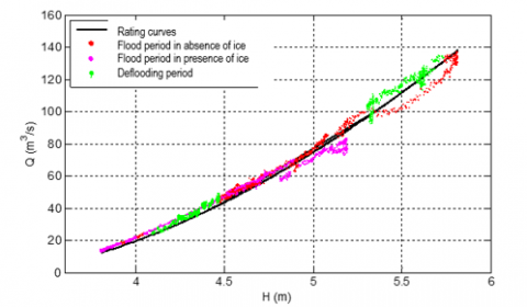
As for the spring flood of 2010, there seems to be a slight hysteresis phenomenon in 2011 (see Figure 7), because the heights recorded during the flood period (red line) are slightly higher than the heights recorded during the deflooding period (green line) for the same flows. The difference between the measured flows and the flows calculated by calibration remains however very small 2.51% and lower than that obtained for the other years.
As in previous years, two rating curves were considered. The rating curve calibrated with the flows measured in the absence of ice produces a 2.59% difference compared to the 2.51% difference obtained with the single rating curve. Furthermore, the deviation obtained in the presence of ice, 2.55%, is slightly higher than that obtained in the absence of ice. This refers to the interpretation that the flow through the ice-covered section of a river can correspond to any ice height [11]. All in all, the overall deviation for all values calculated with the two rating curves is 2.58%.
Figure 7. Rating curves for flood periods in the presence and absence of ice 2011
4.4 Summary of the results obtained with two rating curves at Bostonnais
Table 1 presents the average results obtained following the analysis of the reliability of the rating curves. These results show that they reproduce with good accuracy, the flood flow measurements that the Doppler SW provided for all years at the Bostonnais River. However, it can be seen that the differences between the flows provided by the two rating curves and those measured with the Doppler SW are decreasing from 2008 to 2011. The analysis of the data for the documented years shows that the flows estimated by the rating curves show much less of a drop-off than those measured by Doppler SW. In fact, this is explained by the observation of the failure of the Doppler SW due to prolonged outages. In addition, it can be seen that the missing data from the limnimeter are much less important than those from the Doppler SW. The results obtained by combining the two rating curves are interesting. The average of the overall deviation obtained with the two rating curves is smaller than that obtained with the single rating curve. Thus, hydrometric station managers can safely use the equations of the two combined rating curves to estimate river flows. Of course, the gain is not very great, but this shows that these results can be improved by reducing the uncertainties of the equipment.
Table 1. Summary of the results obtained for Bostonnais
|
Bostonnais river |
2008 |
2009 |
2010 |
2011 |
Average |
|
Gap/deviation with single rating curve |
9.87% |
6.12% |
4.42% |
2.51% |
5.73% |
|
Gap/deviation with rating curve in the presence of ice |
13.65% |
9.18% |
5.37% |
2.55% |
7.68% |
|
Gap/deviation with rating curve in the absence of ice |
6.03% |
4.94% |
2.68% |
2.59% |
4.06% |
|
Overall Gap/deviation with the two curves |
9.51% |
6.44% |
3.58% |
2.58% |
5.53% |
|
Missing measurements Nstd |
0.14% |
0.55% |
1.95% |
0.16% |
0.93% |
|
Missing measurements Nsw |
23.58% |
26.02% |
1.76% |
0.21% |
9.52% |
Table 2. Frequency of Doppler SW and standard limnimeter failures
|
Measurements missing of standard height |
Missing flow measurements from Doppler SW |
||||||
|
Number |
Rate |
Average rate |
Number |
Rate |
Average rate |
||
|
Bostonnais |
2008 |
5002 |
14.24% |
4.98% |
15103 |
42.98% |
28.60% |
|
2009 |
1064 |
3.04% |
4341 |
12.39% |
|||
|
2010 |
635 |
1.81% |
1857 |
5.30% |
|||
|
2011 |
170 |
0.81% |
11242 |
53.72% |
|||
|
Global |
6871 |
4.98% |
32543 |
28.60% |
|||
4.5 The frequency of breakdowns of the Doppler SW and the standard limnimeter
Table 2 presents the frequency of missing data for the standard level meter and the SW Doppler, expressed as an overall percentage of expected data from the site and by year. It can be seen that the overall percentage of missing data for the SW Doppler is 28.60% compared to 4.98% for the standard level used by both rating curves. In spite of the precise data that the SW Doppler can provide, a finding emerges that shows that the tare curves are necessary to complement it. This complementarity comes into play when the SW Doppler returns erroneous or aberrant data or when it stalls. Since the standard limnimeter stalls less than the Doppler SW, it is obvious that the calibrated rating curves will be able to provide reliable data to replace the missing data from the Doppler SW.
The objective of this article was to propose an integrated approach for estimating river flows under ice cover. To do this, it was necessary to show that it was possible to improve the results obtained by a traditional rating curve. This, using validated SW Doppler measurements obtained continuously in the presence and absence of an ice cover. The calibration of a double calibration curve from the measurements provided by the Doppler SW and filtered made it possible to reduce the average relative difference. The methodology proposed in this article was applied to the Bostonnais River in Quebec. The results obtained are satisfactory, because the two combined rating curves better reproduce the flow rates measured by the Doppler SW, compared to the single rating curve. Thus, it becomes possible to replace the aberrant measurements of the Doppler SW and to estimate the missing data in the event of failure of the latter. The differences between the flows calculated by the double rating curve and those measured by the Doppler SW vary between 2.58 and 8.51% depending on the year and for an overall average of 5.03%. However, these results can be further improved by carrying out, for example, a real-time estimation of the flow. To do this, we can attach the rating curve to the Kalman filter. This will make it possible to overcome the weaknesses of the hypothesis of the univocity of the Q-H relation in non-permanent flow. Thus, with a dynamic rating curve, it will be possible to better process the estimation of flows in a situation of non-permanent flow.
[1] Elshamy, M., Loukili, Y., Pomeroy, J.W., Pietroniro, A., Richard, D., Princz, D. (2022). Physically based cold regions river flood prediction in data‐sparse regions: The Yukon River Basin flow forecasting system. Journal of Flood Risk Management, e12835. https://doi.org/10.1111/jfr3.12835
[2] Guay, C., Choquette, Y., Durand, G. (2012). Hydroacoustic Doppler technology: A key element in the improvement of winter hydrometric data quality. Canadian Water Resources Journal/Revue Canadienne des Resources Hydriques, 37(1): 37-46. https://doi.org/10.4296/cwrj3701867
[3] Schmidt, J.H. (2020). Using fast frequency hopping technique to improve reliability of underwater communication system. Applied Sciences, 10(3): 1172. https://doi.org/10.3390/app10031172
[4] Wijayarathne, D.B., Coulibaly, P. (2020). Identification of hydrological models for operational flood forecasting in St. John’s, Newfoundland, Canada. Journal of Hydrology: Regional Studies, 27: 100646. https://doi.org/10.1016/j.ejrh.2019.100646
[5] Tarek, M., Brissette, F.P., Arsenault, R. (2020). Evaluation of the ERA5 reanalysis as a potential reference dataset for hydrological modelling over North America. Hydrology and Earth System Sciences, 24(5): 2527-2544. https://doi.org/10.5194/hess-24-2527-2020
[6] Perret, E., Lang, M., Le Coz, J., Renard, B. (2018). HYDROM A1: Analyse exploratoire des stations hydrométriques susceptibles d'être concernées par un effet d'hystérésis sur la courbe de tarage. Irstea, p. 27. https://hal.inrae.fr/hal-02608481.
[7] Di Baldassarre, G., Montanari, A. (2009). Uncertainty in river discharge observations: A quantitative analysis. Hydrology and Earth System Sciences, 13(6): 913-921. https://doi.org/10.5194/hess-13-913-2009
[8] Pelletier, P.M. (1988). Uncertainties in the single determination of river discharge: A literature review. Canadian Journal of Civil Engineering, 15(5): 834-850. https://doi.org/10.1139/l88-109
[9] Khalafzai, M.A.K., McGee, T.K., Parlee, B. (2019). Flooding in the James Bay region of northern Ontario, Canada: Learning from traditional knowledge of Kashechewan First Nation. International Journal of Disaster Risk Reduction, 36: 101100. https://doi.org/10.1016/j.ijdrr.2019.101100
[10] Ragot, J., Darouach, M., Maquin, D., Bloch, G. (1990). Validation de données et diagnostic. Hermès Science Publications.
[11] Turcotte, B., Morse, B., Anctil, F. (2012). Hydraulic and hydrological regime of ice-affected channels at freezeup. Cold Regions Engineering, 242-252. http://dx.doi.org/10.1061/9780784412473.024
[12] Lamarche, O., Hébert, S. (2020). Géologie des dépôts de surface de la région de la rivière Eastmain supérieure (SNRC 23D05, 23D06, 23D11, 23D12, 33A08 à 33A10). Document publié par la Direction générale de Géologie Québec.
[13] Cornford, S.L., Seroussi, H., Asay-Davis, X.S., et al., (2020). Results of the third marine ice sheet model intercomparison project (MISMIP+). The Cryosphere, 14(7): 2283-2301. https://doi.org/10.5194/tc-14-2283-2020
[14] Namaee, M.R., Sui, J.Y. (2020). Velocity profiles and turbulence intensities around side-by-side bridge piers under ice-covered flow condition. Journal of Hydrology and Hydromechanics, 68(1): 70-82. https://doi.org/10.2478/johh-2019-0029
[15] Robert, A., Tran, T. (2012). Mean and turbulent flow fields in a simulated ice‐covered channel with a gravel bed: some laboratory observations. Earth Surface Processes and Landforms, 37(9): 951-956. https://doi.org/10.1002/esp.3211
[16] Rokaya, P., Peters, D.L., Bonsal, B., Wheater, H., Lindenschmidt, K.E. (2019). Modelling the effects of climate and flow regulation on ice‐affected backwater staging in a large northern river. River Research and Applications, 35(1): 587-600. http://dx.doi.org/10.1002/rra.3436
[17] Morse, B., Turcotte, B. (2018). Risque d’inondations par embâcles de glaces et estimation des débits hivernaux dans un contexte de changements climatiques (Volet A). Rapport présenté à Ouranos.
[18] Turcotte, R., Favre, A.C., Lacombe, P., Poirier, C., Villeneuve, J.P. (2005). Estimation des débits sous glace dans le sud du Québec: Comparaison de modèles neuronal et déterministe. Canadian Journal of Civil Engineering, 32(6): 1039-1050. http://dx.doi.org/10.1139/l05-084
[19] CR, A., Thatikonda, S. (2020). Study on backwater effect due to Polavaram Dam Project under different return periods. Water, 12(2): 576. https://doi.org/10.3390/w12020576
[20] Hidayat, H., Vermeulen, B., Sassi, M., Torfs, P., Hoitink, A. (2011). Discharge estimation in a backwater affected meandering river. Hydrology and Earth System Sciences, 15(8): 2717-2728. https://doi.org/10.5194/hess-15-2717-2011
[21] Petersen‐Øverleir, A., Reitan, T. (2009). Bayesian analysis of stage-fall-discharge models for gauging stations affected by variable backwater. Hydrological Processes: An International Journal, 23(21): 3057-3074. https://doi.org/10.1002/hyp.7417
[22] Lachance-Cloutier, S., Turcotte, R., Cyr, J.F. (2017). Combining streamflow observations and hydrologic simulations for the retrospective estimation of daily streamflow for ungauged rivers in southern Quebec (Canada). Journal of Hydrology, 550: 294-306.
[23] Guo, Y.H., Zhang, Y.Q., Zhang, L., Wang, Z.G. (2021). Regionalization of hydrological modeling for predicting streamflow in ungauged catchments: A comprehensive review. Wiley Interdisciplinary Reviews: Water, 8(1): e1487. https://doi.org/10.1002/wat2.1487
[24] Brunner, M.I., Melsen, L.A., Newman, A.J., Wood, A. W., Clark, M.P. (2020). Future streamflow regime changes in the United States: Assessment using functional classification. Hydrology and Earth System Sciences, 24(8): 3951-3966. https://doi.org/10.5194/hess-24-3951-2020
[25] Jiang, Q.J., Qi, Z.M., Tang, F., Xue, L.L., Bukovsky, M. (2020). Modeling climate change impact on streamflow as affected by snowmelt in Nicolet River Watershed, Quebec. Computers and Electronics in Agriculture, 178: 105756. https://doi.org/10.1016/j.compag.2020.105756
[26] Muste, M., Kim, W., Fulford, J.M. (2008). Techniques hydrométriques: Perfectionnement des instruments pour la cartographie hydrodynamique des cours d’eau. Bulletin de l’OMM, 57(3): 163.
[27] Hamilton, S. (2003). Winter Hydrometry: Real-time data issues. In Proceedings of the 12th Workshop on the Hydraulics of Ice Covered Rivers, Edmonton, Canada. http://cripe.ca/docs/proceedings/12/Hamilton-2003.pdf, accessed on 20 July 2020.
[28] Morlot, T., Perret, C., Favre, A.C., Jalbert, J. (2014). Dynamic rating curve assessment for hydrometric stations and computation of the associated uncertainties: Quality and station management indicators. Journal of Hydrology, 517: 173-186. https://doi.org/10.1016/j.jhydrol.2014.05.007
[29] Mansanarez, V., Renard, B., Coz, J.L., Lang, M., Darienzo, M. (2019). Shift happens! Adjusting stage‐discharge rating curves to morphological changes at known times. Water Resources Research, 55(4): 2876-2899. https://doi.org/10.1029/2018WR023389
[30] Danial, M.M., Kawanisi, K., Al Sawaf, M.B. (2019). Characteristics of tidal discharge and phase difference at a tidal channel junction investigated using the fluvial acoustic tomography system. Water, 11(4): 857. https://doi.org/10.3390/w11040857
[31] Mballa, E.L., Bennis, S. (2015). Analyse de l’opportunité d’application des méthodes d’estimation des débits des rivières par courbe de tarage et capteur doppler immergé fixe. Canadian Journal of Civil Engineering, 42(5): 329-341. https://doi.org/10.1139/cjce-2013-0509