Jayalakshmi Pothala | Obulesu Mopuri | Charankumar Ganteda | Madhu Mohan Reddy Peram | Gangadhar Kotha | Giulio Lorenzini*
© 2022 IIETA. This article is published by IIETA and is licensed under the CC BY 4.0 license (http://creativecommons.org/licenses/by/4.0/).
OPEN ACCESS
In this article, an analysis of magnetohydrodynamic fluid flow in addition to heat transfer involving a nanofluid flowing through a stretched cylinder has been performed in the being there of Newtonian heating. In the heating and cooling processing sectors, Newtonian heating is particularly essential. Utilizing similarity transformations, in the absence of appropriate boundary conditions, ordinary differential equations are a collection of equations that are used to solve problems (ODE) corresponds to the governing partial differential equations (PDE), The Runge-Kutta-Gill technique and the shooting strategy are then used to numerically solve the problems. Water has been used as the foundation fluid for a variety of nanoparticles, including Copper (Cu), Silver (Ag), Alumina (Al2O3), and Titanium Oxide (TiO2). The present results used for the surface Shear stress and the local Nusselt number are in very good agreement with those previously published. Advanced skin friction coefficients and heat transfer rates were found to be increased with M and Re valued higher. In addition, copper (for a small amount of magnetic parameter) and alumina (for a large amount of magnetic parameter) the optimum cooling materials for this problem have also been found.
stretching cylinder, nanoparticles, MHD, Newtonian heating
It is highly known that Choi [1] was the primary to use the word the phrase "nanofluid," which refers to a fluid in which nanoscale particles are suspended in a low-thermal-conductivity base fluid such as water, ethylene glycol, or oils etc. [2]. The notion of nanofluid has been advocated in recent years as a way to improve upon the existing presentation of heat transport rates in liquids. Nanomaterials are materials with dimensions on the nanoscale scale have only one of its kind physical and chemical characteristics [3]. Since they are tiny sufficient to perform like liquid molecules, they can flow freely through micro-channels without blocking them [4]. This fact has piqued the interest of numerous scholars, including [5-16] They investigated the heat transfer properties of nanofluids and observed that when nano particles are present, the fluid's effective thermal conductivity rises dramatically, improving heat transfer characteristics. This is a fantastic compilation of papers on the subject. Be able to be establish in the references [17-22], with in the volume written by Das et al. [4].
The boundary conditions that are generally utilised for modelling the border line sheet stream and warmth transfer of stretching/shrinking surfaces are moreover a given exterior warmth or a specified exterior warmth flux. Though, boundary layer heat transfer is affected by surface temperature in border line layer flood as well as heat transfer issues. The graph below shows an example of surface heat transmission and temperature have a linear connection. This condition occurs, for example, in conjugate heat transport issues (see [23]), and when convective fluid on the surface is heated Newtonian; the latter condition was examined in detail in by Merkin [24]. As a result of conjugate convection, the convective fluid is provided with heat via a boundary a heat-conducting surface having a limited capacity. While a result, the rate of heat transport from side to side the exterior is proportional to the temperature in the area differential because to the surrounding conditions. Many essential technical equipment use this Newtonian heating set of connections, such as warmth exchangers, wherever the transference throughout a tube with a solid wall is substantially impacted by the flow of fluid passing across it convects. With a convective boundary condition, there are issues about heat transmission for boundary layer flow, on the other hand, have lately been explored by Aziz [25], Makinde and Aziz [26], Ishak [27], and Magyari [28] for the Blasius flow. With radiation impacts, a similar analysis was performed on the Blasius and Sakiadis rivers by Bataller [29]. Yao et al. [30] Recently, researchers investigated the heat transfer of a viscous fluid flow through a permeable stretching/shrinking sheet with a convective boundary condition. Magyari and Weidman [31] together Based on a defined exterior temperature as well as arranged exterior heat flux, the heat transfer properties of a semi-infinite flat plate owing to a uniform shear flow were studied. It's worth noting that a consistent shear flow is propelled greater than the protect by a viscous on the outside flow through rotating velocity, whereas a classical Blasius flow is propelled in excess of the shield by an inviscid on the outside pour with irrotational velocity.
In physics, chemistry, and engineering, the investigation of magnetic field effects is essential. Electrically conducting fluids and electromagnetic fields are often used together to MHD generators, pumps, bearings, and border line layer control systems are all being developed. Regarding these applications, various investigators' work has been reviewed. The hydromagnetic behaviour of border line layers the length of surfaces that do not change or surfaces that move in the attendance of an oblique magnetic field is one of the most primary and indispensable questions in this regulation. MHD border line layers have been seen in a variety of scientific systems that make use of fluid metal and plasma flood in excess of magnetic fields [32]. Newly, In the presence of a magnetic field, scientists have looked into the effects of Electrically conducting fluids are fluids that are incompressible, viscous, and flow over a surface or stretched plate, metals that are liquid, water combined with a touch of acid, and other compounds. Pavlov [33] was one of the most important forerunners in the field of education. In the presence of a transverse magnetic field, the moving flow of a flat plate or sheet became such an attractive issue after Pavlov's research that it spawned a considerable body of literature. A two-dimensional MHD stagnation point's migration towards a stretched component has been studied as a function of changing outside temperature by Ishak et al. [34]. when the stretching velocity is greater than the free of charge stream velocity, they discovered that the surface heat transfer rate increases with the magnetic parameter, i.e. $\varepsilon>1$ and the opposite is observed when $\varepsilon<1$ . Study of the effects of when the stretching velocity is higher than the velocity of the free-flowing stream by Hamad et al. [35]. Cu and Ag nanoparticles, they find, offer under this case, the optimum cooling performance. Their impact, on the other hand, is minor. Devi and Thiyagarajan [36] Researchers in a changing transverse magnetic field, with heat transfer across a variable temperature surface, the incompressible, viscous, and electrically conducting flow of a continuous nonlinear hydromagnetic flow fluid extends by means of a power-law velocity. Kumaran et al. [37] the changeover of the movement of MHD boundary layers past a stretched sheet was studied. Their findings show that when the magnetic field parameter increases, the wall temperature profile falls dramatically. Furthermore, when the magnetic component of the flow characteristics increases, the skin friction of the sheet decreases. Prasad et al. [38] Variable viscosity has an influence on Heat transmission and viscoelastic fluid flow in MHD across a stretched sheet. According to their analysis, when the magnetic parameter of the flow characteristics increases, the sheet's skin friction decreases. Hot rolling, wire drawing, glass–fiber and paper production, plastic film drawing, metal and polymer extrusion, metal spinning, and liquid films in the condensation process are only a few examples of technological applications, etc. [39]. Ashorynejad et al. [40] a stretched cylinder was used to investigate magnetic fields and their effects on nanofluid flow and heat transfer. Copper (Cu), Silver (Ag), Alumina (Al2O3), and Titanium oxide (TiO2) were explored, with water as the base fluid. Mutuku and Makinde [41] the effects of MHD on a nanofluid heat and mass transfer flow across an unstable flat surface were explored. Khanet et al. [42] over a stretched sheet, researchers investigated the effects of MHD and Newtonian heating on the Powell-Eyring fluid. It was discovered that increasing the conjugate parameter of Newtonian heating improves the rate of heat transfer. Gangadher et al. [43] the effect of in a permeable stretching shrinking sheet, Newtonian heating is applied to a micropolar nanofluid was investigated. Copper (Cu), Alumina (Al2O3), and Titanium oxide (TiO2) were studied in water-based nanofluids.
The current study was prompted by the aforementioned findings, which revealed that the majority of the issues are related to nanofluids heated by Newtonian heating on a sheet, stretched surface, or flat plate. However, the research of Newtonian heating by a magneto hydrodynamic nanofluid flow across a stretched cylinder has not yet been addressed, to the author's knowledge. The Keller Box technique is used to solve the converted ordinary differential equations numerically. The findings of select rare situations are computed and compared to the current results, yielding a remarkable agreement.
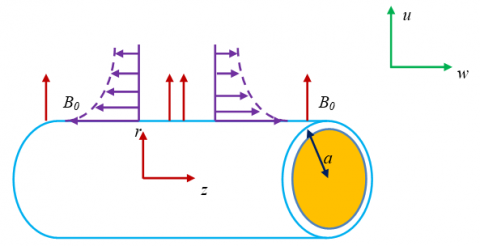
In an electrically conducting fluid that is incompressible (with electrical conductivity) at rest, consider laminar nanofluid flow as shown in Figure 1, Z-axis is calculated the length of the tube's axis, while R-axis is measured in radial direction. The cylinder's surface is supposed to be subject to a Newtonian heating boundary condition. The ambient solution high temperature is given by $T_{\infty}$. As well as the uniform magnetic field has a radial intensity $B_0$ and so as to if because the magnetic Reynolds number is small, the magnetic field has minimal effect.
Figure 1. The coordinate system and the physical model
It is excluded the effects of Hall effect, viscous dissipation, and Ohmic heating, since they are also believed to be minor. The field consists of a watery fluid containing a number of nanoparticles: Cu, Al2O3, Ag and TiO2. As far as thermal equilibrium is concerned, the base fluid and the nanoparticles are in agreement. Table 1 lists the thermo physical parameters of the nanofluid [9]. Considering these assumptions, the nanofluid model below was developed by Tiwari and Das [6], the governing equations are (see [44-46]).
$\frac{\partial(r w)}{\partial z}+\frac{\partial(r u)}{\partial r}=0$ (1)
$\rho_{n f}\left(w \frac{\partial w}{\partial z}+u \frac{\partial u}{\partial r}\right)=\mu_{n f}\left(\frac{\partial^2 w}{\partial r^2}+\frac{1}{r} \frac{\partial w}{\partial r}\right)-\sigma_{n f} B_0{ }^2 w$ (2)
$\rho_{n f}\left(w \frac{\partial u}{\partial z}+u \frac{\partial u}{\partial r}\right)=-\frac{\partial p}{\partial r}+\mu_{n f}\left(\frac{\partial^2 u}{\partial r^2}+\frac{1}{r} \frac{\partial u}{\partial r}-\frac{u}{r^2}\right)$ (3)
$w\frac{\partial T}{\partial z}+u\frac{\partial T}{\partial r}=\frac{{{k}_{nf}}}{{{(\rho {{C}_{p}})}_{nf}}}\left( \frac{{{\partial }^{2}}T}{\partial {{r}^{2}}}+\frac{1}{r}\frac{\partial T}{\partial r} \right)$ (4)
Subject to the boundary conditions
$u={{u}_{w}}$,$w={{w}_{w}}$,$\frac{\partial T}{\partial r}=-{{h}_{s}}T$ at $r=a$ $w\to 0$,$T\to {{T}_{\infty }}$ as $r\to \infty $ (5)
On the r, we have u and w, which are velocity components and z – axes, in that order, and ${{w}_{w}}=2cz$, where $c$ a positive constant is and T is the fluid temperature. The effective density ${{\rho }_{nf}}$, the effective dynamic viscosity ${{\mu }_{nf}}$, ${{h}_{s}}$ the heat transfer parameter for Newtonian heating, the heat capacitance ${{\left( \rho Cp \right)}_{nf}}$, the thermal conductivity of the nanofluid ${{k}_{nf}}$ and ${{\sigma }_{nf}}$ the conductivity of the fluid are given as [47]:
${{\rho }_{nf}}=(1-\varphi ){{\rho }_{f}}+\varphi {{\rho }_{s}}$, ${{\mu }_{nf}}=\frac{{{\mu }_{f}}}{{{\left( 1-\varphi \right)}^{2.5}}}$, ${{(\rho {{C}_{p}})}_{nf}}=(1-\varphi ){{(\rho {{C}_{p}})}_{f}}+\varphi {{(\rho {{C}_{p}})}_{s}}$, ${{\sigma }_{nf}}=(1-\varphi ){{\sigma }_{f}}+\varphi {{\sigma }_{s}}$, $\frac{{{k}_{nf}}}{{{k}_{f}}}=\frac{{{k}_{s}}+2{{k}_{f}}-2\varphi ({{k}_{f}}-{{k}_{s}})}{{{k}_{s}}+2{{k}_{f}}+2\varphi ({{k}_{f}}-{{k}_{s}})}$ (6)
where, $\varphi$ is the solid volume fraction.
Following Wang [44] we take the similarity transformations:
$\eta ={{(r/a)}^{2}}$, $u=-ca\left( f(\eta )/\sqrt{\eta } \right)$,$w=2c{f}'(\eta )z$, $\theta (\eta )=(T-{{T}_{\infty }})/{{T}_{\infty }}$ (7)
where prime signifies a distinction in terms of $\eta$.
The ordinary differential equations are as follows when Eqns. (2) and (4) are plugged into Eq. (7):
$\operatorname{Re}.{{A}_{1}}.{{(1-\varphi )}^{2.5}}({{{f}'}^{2}}-f{f}'')$$=\eta {f}''+{f}''-M.{{(1-\varphi )}^{2.5}}{f}'$ (8)
$\eta {\theta }''+(1+\operatorname{Re}\Pr f{{A}_{2}}/{{A}_{3}}){\theta }'=0$ (9)
The boundary conditions (5), in addition to the border line conditions (4), become
$f(1)=0$, ${f}'(1)=1$, $\theta (1)=-{\theta }'(1)/\gamma -1$ (10)
$f^{\prime}(\infty) \rightarrow 0, \quad \theta(\infty) \rightarrow 0$ (11)
Here $\operatorname{Re}=c{{a}^{2}}/2{{v}_{f}}$ is the Reynolds number, $M={{\sigma }_{nf}}{{B}_{0}}^{2}{{a}^{2}}/(4{{\mu }_{f}})$ is the magnetic parameter, $\gamma ={{h}_{s}}{{a}^{2}}/2r$ is the Newtonian heating parameter, $\Pr ={{\mu }_{f}}{{(\rho {{C}_{p}})}_{f}}/({{\rho }_{f}}{{k}_{f}})$ is the Prandtl number and the constants A1, A2, and A3 are given by:
${{A}_{1}}=(1-\phi )+\frac{{{\rho }_{s}}}{{{\rho }_{f}}}\phi $,${{A}_{2}}=(1-\phi )+\frac{{{(\rho {{C}_{p}})}_{s}}}{{{(\rho {{C}_{p}})}_{f}}}\phi $, ${{A}_{3}}=\frac{{{k}_{nf}}}{{{k}_{f}}}=\frac{{{k}_{s}}+2{{k}_{f}}-2\phi ({{k}_{f}}-{{k}_{s}})}{{{k}_{s}}+2{{k}_{f}}+2\phi ({{k}_{f}}-{{k}_{s}})}$ (12)
Eq. (3) may now be used to calculate the pressure in the manner.
$\frac{P-P_{\infty}}{\rho_{n f}\quad c v_{n f}}=-\frac{\operatorname{Re}}{\eta} \cdot A_1 \cdot(1-\varphi)^{2.5} f^2(\eta)-2 f^{\prime}(\eta)$ (13)
Two key physical variables are the skin friction coefficient and the Nusselt number Nu. ${{C}_{f}}=\frac{{{\tau }_{w}}}{{{\rho }_{f}}{{w}_{w}}^{2}}$,
$Nu=\frac{a{{q}_{w}}}{{{k}_{f}}({{T}_{w}}-{{T}_{\infty }})}$ (14)
where, ${{\tau }_{w}}$ and ${{q}_{w}}$ are respectively, skin friction and heat transfer from the cylinder's surface, and they are given by
${{\tau }_{w}}={{\mu }_{nf}}{{\left( \frac{\partial w}{\partial r} \right)}_{r=a}}$, ${{q}_{w}}=-{{k}_{nf}}{{\left( \frac{\partial T}{\partial r} \right)}_{r=a}}$ (15)
$(2z\operatorname{Re}/a){{C}_{f}}=\frac{1}{{{(1-\varphi )}^{2.5}}}{f}''(1)$, $Nu=-2\frac{{{k}_{nf}}}{{{k}_{f}}}{\theta }'(1)$ (16)
The present situation's governing equations are converted keen on a collection of connected using similarity transformations to crack nonlinear differential equations. The Runge-Kutta-Gill technique and the gunshot approach are used to numerically integrate the Eqns. (8)-(9) as well as the boundary conditions (10)-(11). In comparison to other Runge-Kutta equations, the Runge-Kutta-Gill technique compensates for cumulative round-off error while utilising less storage. (Kumar and Unny [48]). The following is a succinct description of this procedure:
$\begin{align} & {{y}_{1}}=f,\,\,{{y}_{2}}={f}',\,\,{{y}_{3}}={{f}'}',\,{{y}_{4}}=\,\theta ,\,\,{{y}_{5}}={\theta }' \\ & {{y}_{3}}^{\prime }\,=\,\frac{1}{\eta }\operatorname{Re}\,{{(1-\Phi )}^{2.5}}\left[ {{y}_{2}}^{2}-{{y}_{1}}{{y}_{3}} \right]-\frac{1}{\eta }\left[ {{y}_{3}}-Mn\,{{(1-\Phi )}^{2.5}}\,{{y}_{2}} \right] \\ & {{y}_{5}}^{\prime }\,=\,-\frac{1}{\eta }\left[ 1+\operatorname{Re}\Pr {{y}_{1}}\frac{{{A}_{2}}}{{{A}_{3}}} \right]{{y}_{5}} \\\end{align}$ (17)
The boundary conditions are changed in the following way:
$\begin{align} & {{y}_{1}}(1)=S,\,\,\,{{y}_{2}}(1)=-1,\,\,{{y}_{4}}(1)=-\frac{{{y}_{5}}(1)}{\gamma }-1 \\ & {{y}_{2}}(\infty )\to 0,\,\,\,{{y}_{4}}(\infty )\to 0 \\\end{align}$ (18)
To complete the Integration of the equations in a step-by-step manner (9) – (10), The techniques developed by Gill include employed (Ralston and Wilf [49]). To begin the integration, all of the values of must be provided $y_1, y_2, y_3, y_4, y_5, y_6$ at $\eta=0$ as of which vantage point, although forward integration has been performed, it is clear the values are derived from the boundary conditions are not equal of $y_3, y_4, y_7$ are not known. As a result, we must offer such values of $y_3, y_4, y_7$ as well as the other function's known values at $\eta=0$ as long as the boundary criteria are met as following step-by-step integrations, to a predetermined accuracy. Because of the significance of $y_3, y_4, y_7$ Because the numbers provided are only approximate estimates, certain adjustments must be done to ensure that the boundary criteria are met to $\eta \rightarrow \infty$ are contented. These adjustments to the values of $y_3, y_4, y_7$ are taken care of by a self-iterative treatment that may be referred to as a remedial operation for convenience.
The Runge-Kutta-Gill technique and the shot approach were used to (7) and (8) are nonlinear ordinary differential equations that need to be solved numerically, using boundary conditions (10) – (11). With water as the basic fluid, we used four different types of nanoparticles: Copper (Cu), Silver (Ag), Alumina (Al2O3), and Titanium oxide (TiO2). The thermophysical characteristics of the base fluid water and nanoparticles Cu, Ag, Al2O3, and TiO2 were shown in Table 1. The fundamental fluid is (water), the Prandtl number is maintained at the same level at 7. It's worth noting that the results of this research are reduced compared to the properties of a viscous or ordinary fluid when $\Phi$ =0.
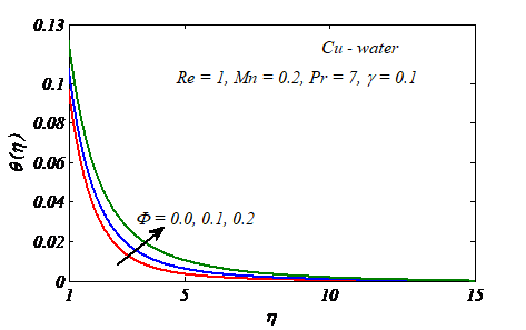
Figure 2 depicts the temperature curve for many nanoparticals. The temperature profile may be seen for nano particles rises progressively from the stretched sheet's surface. Ag-water nanofluid fluid temperatures are lower than Cu-water, Al2O3-water, and TiO2-water nanofluid fluid temperatures. Because the thermal conductivity of Silver (Ag) is higher than that of Copper (Cu), Alumina (Al2O3), and Titanium oxide, the physics underpinning this conclusion is correct (TiO2). In the instance of Cu nanoparticles and water base fluid (Pr =7), Figures 3 and 4 demonstrate how the volume percentage of nanoparticles affects the velocity and temperature profiles of nanofluids, respectively when $\Phi $= 0, 0.1 and 0.2 with Mn = 0.2, $\gamma $ = 0.1, Re = 1. The nanofluid velocity decelerates as the volume percentage of nanoparticales increases, while the temperature rises. This aggression with physical action is depicted in these figures. The thermal conductivity layer grows as the volume of nanoparticles grows. Figure 5, 6 and 7 illustrate the effect of transverse magnatic field parameter Mn on nanofluid velocity ${f}'(\eta )$, pressure distribution $(P-{{P}_{\infty }})/({{\rho }_{nf}}c\,{{\nu }_{nf}})$ and temperature distribution $\theta (\eta )$ respectively.
Figure 2. Temperature profiles $\theta(\eta)$ for various nanoparticle kinds
Figure 3. Velocity profiles ${f}'(\eta )$ under dissimilar principles of nanoparticle volume fraction $\Phi $
Table 1. Water and nanoparticles' thermophysical characteristics [9]
|
|
$\rho \,(kg/{{m}^{3}})$ |
${{c}_{p}}\,\,(j/kg\,\,K)$ |
$k\,(W/m\,K)$ |
$\beta \times {{10}^{5}}\,({{K}^{-1}})$ |
|
Pure water Copper (Cu) Silver (Ag) Alumina (Al2O3) Titanium oxide (TiO3) |
997.1 8.933 10.500 3.970 4.250 |
4.179 385 235 765 686.2 |
0.613 401 429 40 8.9538 |
21 1.67 1.89 0.85 0.9 |
Figure 4. Temperature profiles $\theta (\eta )$ for various nanoparticle volume fraction values $\Phi $
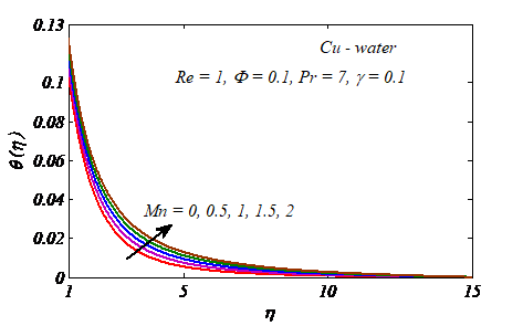
Figure 5 show that as the magnetic field parameter Mn is increased, the nanofluid velocity decreases in the case of Cu-water when Mn= 0, 0.5, 1, 1.5 and 2, with Re = 1, $\Phi $= 0.1, Pr = 7 and $\gamma $ = 0.1. The transverse magnatic field, as shown, obviously resists the transport event. This is owing to the fact that changes in Mn cause changes in the Lorentz force as a result of the magnatic field, and Transport events are made more difficult by the Lorentz force. The velocity vanishes at a significant distance from the cylinder's surface in all situations. Figure 6 further shows that when the parameter Mn rises, the pressure increases. Thus, the location in which $P\to {{P}_{\infty }}$ placed further from the surface of the cylinder. This conclusion is in agreement with those of Ashorynejad et al. [40]. The temperature of the nanofluid discovered inside the cylinder rises, eventually reaching a great distance from the cylinder's surface (Figure 7). As a result of the increased magnatic field strength, the thickness of as seen in table [7], the thermal boundary layer expands, reducing the Nusselt number. The effect of Newtonian heating parameter $\gamma $on temperature profile in the case of Cu-water when the conjugate parameter for Newtonian heating $\gamma $ = 0 (in the absence of Newtonian heating), 0.01, 0.02, 0.03, 0.04 and 0.05 with Re = 1, $\varphi $= 0.1, Mn = 0.2, Pr = 7 is shown in Figure 8. It is clear that the temperature distribution increases with an increase in the Newtonian heating parameter$\gamma $. As $\gamma \to \infty $, The wall temperature scenario was defined by the Newtonian heating condition. It's also worth noting that the temperature of nanofluids goes to zero as $\gamma $= 0. The conjugate heat transfer coefficient is exactly proportional to the Newtonian heating parameter. When the Newtonian heating parameter is increased and the temperature rises, the conjugate heat transfer coefficient increases.
Figure 5. Distinct values of the magnetic field parameter M result in different velocity patterns $f^{\prime}(\eta)$
Figure 6. Pressure distribution $P-P_{\infty} / \rho_{n f} c v_{n f}$ under different values of magnetic field parameter Mn
Figure 7. Temperature profiles $\theta(\eta)$ for various magnetic field parameter values $M n$
Figure 8. Temperature profiles $\theta(\eta)$ for various Newtonian heating parameter values $\gamma$
Figure 9 and 10 displace the behavior of the skin fraction coefficient and Nusselt number for various values of nanopartical volume fraction $\Phi $ and Reynolds number Re when Mn = 0.2, Pr = 7, and $\gamma $= 0.1. It's worth noting that the Reynolds number Re shows how important the inertia impact is in comparison to the viscous effect. As a result, raising Re raises the size of the skin fraction coefficient and the Nusselt number. The same behavior was observed with an increase in nanopartical volume fraction. The present results are juxtaposed with Ishak et al. [50] and Wang [44], Briefly, Ishak et al. [50] The effect of magnetic field strength on flow across a stretched cylinder and heat transfer treatment was investigated. Wang [44] the fluid flow caused by a stretched cylinder was explored. The stretched cylinder in this issue has a constant temperature and linear velocity.
Figure 9. Skin friction coefficient $-\frac{1}{{{\left( 1-\Phi \right)}^{2.5}}}{{f}'}'(1)$ under different values of $\operatorname{Re}\,\,\And \,\,\Phi $
Figure 10. Local Nusselt number $-\frac{{{k}_{nf}}}{{{k}_{f}}}{\theta }'(1)$ under different values of $\operatorname{Re}\,\,\And \,\,\Phi $
Table 2. Comparison of the skin friction coefficient $f^{\prime \prime}(1)$ for several values of M when Re=10 for clear fluids
|
M |
Present out comes |
Ishak et al. [50] |
Wang [44] |
|
0 0.01 0.05 0.1 0.5 1 2 5 |
-3.344457 -3.346147 -3.352894 -3.361297 -3.427427 -3.507691 -3.661549 -4.082633 |
-3.3444 -3.3461 -3.3528 -3.3612 -3.4274 -3.5076 -3.6615 -4.0825 |
-3.34445 |
Tables 2-5 reported the comparison of skin friction coefficient ${f}''\left( 1 \right)$ and the Nusselt number ${\theta }'\left( 1 \right)$ with published results. The present solutions are compared with the Ishak et al. [50] and Wang [44] and found good convergence with their solutions. Tables 6 and 7 show how different nanofluids affect the Nusselt number and skin friction coefficient. When different types of nanofluid are utilised, the skin friction coefficient and Nusselt number change, as shown in the tables. This means that the sort of nanofluids used in cooling and heating operations will be crucial. For all values of the magnetic parameter Mn, it is also discovered that, picking alumina as the nanoparticle results in the highest skin friction coefficient, whilst choosing silver results in the lowest. For small values of Mn, when copper is used as the nanoparticle, the Nusselt number is maximised, however when alumina is used, the Nusselt number is maximised for large values of Mn. It can also be noticed that choosing titanium oxide results in the least amount of Nusselt number [51-53].
Table 3. Comparison of the Nusselt number $-{\theta }'(1)$ for several values of M and Pr when Re=10,$\gamma \to \infty $ for clear fluids
|
M |
Pr=0.7 (air) |
Pr=7 (water) |
||||
|
|
Present out comes |
Ishak et al. [50] |
Wang [44] |
Present out comes |
Ishak et al. [50] |
Wang [44] |
|
0 0.01 0.05 0.1 0.5 1 2 5 |
1.568110 1.567671 1.565924 1.563760 1.547066 1.527400 1.491038 1.398393 |
1.5687 1.5683 1.5665 1.5644 1.5478 1.5284 1.4924 1.4012 |
1.568 |
6.157997 6.157610 6.156065 6.154142 6.139030 6.120726 6.085700 5.989989 |
6.1592 6.1588 6.1573 6.1554 6.1402 6.1219 6.0864 5.9855 |
6.160 |
Table 4. Comparison of the skin friction coefficient $f^{\prime \prime}(1)$ for several values of M, Re for clear fluids
|
M |
Re=1 |
Re=5 |
||||
|
|
Present out comes |
Ishak et al. [50] |
Wang [44] |
Present out comes |
Ishak et al. [50] |
Wang [44] |
|
0 0.01 0.05 0.1 0.5 |
-1.178005 -1.183890 -1.206846 -1.234424 -1.426925 |
-1.1780 -1.1839 -1.2068 -1.2344 -1.4269 |
-1.17776 |
-2.417437 -2.419887 -2.429641 -2.441734 -2.535233 |
-2.4174 -2.4199 -2.4296 -2.4417 -2.5352 |
-2.41745 |
Table 5. Comparison of the Nusselt number $-{\theta }'(1)$for several values of M and Re when Pr = 7, $\gamma \to \infty $ for clear fluids
|
M |
Re=1 |
Re=100 |
||||
|
|
Present out comes |
Ishak et al. [50] |
Wang [44] |
Present out comes |
Ishak et al. [50] |
Wang [44] |
|
0 0.01 0.05 0.1 0.5 |
2.058751 2.057302 2.051665 2.044918 1.998065 |
2.0587 2.0572 2.0516 2.0449 1.9978 |
2.059 |
19.118511 19.118397 19.117944 19.117377 19.112851 |
19.1587 19.1586 19.1581 19.1576 19.1530 |
19.12 |
Table 6. Effects of the magnetic parameter for different types of nanofluids on skin friction coefficient when Pr =7,$\Phi =0.1,\,\,\gamma =0.1$, Re=1
|
M |
Nanoparticles |
|||
|
Cu |
Ag |
Al2O3 |
TiO2 |
|
|
0 1 5 10 |
-1.762717 -2.174508 -3.270312 -4.223613 |
-1.828320 -2.226299 -3.303665 -4.249074 |
-1.533377 -2.000561 -3.162176 -4.141877 |
-1.547375 -2.010824 -3.168382 -4.146534 |
Table 7. Effects of the magnetic parameter for different types of nanofluids on Nusset number when Pr =7,$\Phi =0.1,\,\,\gamma =0.1$, Re=1
|
M |
Nanoparticles |
|||
|
Cu |
Ag |
Al2O3 |
TiO2 |
|
|
0 1 5 10 |
0.091021 0.090342 0.088558 0.087257 |
0.090823 0.090144 0.088365 0.087076 |
0.091348 0.090625 0.088751 0.087400 |
0.091548 0.090864 0.089058 0.087726 |
This research looked at the continuous electrically conductive nanofluid flowing in two dimensions over a stretched cylindrical pipe due to Newtonian heating. The basic equations regulating flow and heat transmission were simplified to ordinary differential equations are a collection of equations that are used to solve problems by employing the stable temperature and velocity transformation. The Runge-Kutta-Gill method and the shot approach are used to solve these equations numerically. On heat and flow transmission parameters, the impacts of nanoparticle volume fraction, nanofluid type, magnetic field intensity, Reynolds number, and Newtonian heating were investigated. The following are some of the findings of this investigation:
a) The transverse magnetic field suppresses the velocity field, causing the skin fraction coefficient to increase.
b) The magnetic field outcome is to be speed up the nanofluid heat field, which in turn causes the decrement of the Nusselt number.
c) The Newtonian heating causes the increment in both temperature and nanofluid heat transfer rate.
d) Choosing silver for high amount of Newtonian heating leads to high heating performance founded.
e) Copper (for a high quantity of magnetic parameter) and alumina provide the best cooling performance for this situation (for a high amount of magnetic parameter).
[1] Choi, S.U.S., Eastman, J.A. (1995). Enhancing thermal conductivity of fluids with nanoparticles. The Proceedings of the 1995 ASME International Mechanical Engineering Congress and Exposition, San Francisco, USA. ASME, FED 231/MD 66 1995, pp. 99-105.
[2] Wang, X.Q., Mujumdar, A.S. (2007). Heat transfer characteristics of nanofluids: A review. Int J Therm Sci., 46(1): 1-19. https://doi.org/10.1016/j.ijthermalsci.2006.06.010
[3] Das, S.K., Choi, S.U.S., Yu, W., Pradeep, T. (2007). Nanofluids: Science and Technology NJ: Wiley.
[4] Khanafer, K., Vafai, K., Lightstone, M. (2003). Buoyancy-driven heat transfer enhancement in a two-dimensional enclosure utilizing nanofluids. Int J Heat Mass Transfer, 46(19): 3639-3653. https://doi.org/10.1016/S0017-9310(03)00156-X
[5] Abu-Nada, E. (2008). Application of nanofluids for heat transfer enhancement of separated flows encountered in a backward facing step. Int J Heat Fluid Flow, 29(1): 242-249. https://doi.org/10.1016/j.ijheatfluidflow.2007.07.001
[6] Tiwari, R.J., Das, M.K. (2007). Heat transfer augmentation in a two-sided lid-driven differentially heated square cavity utilizing nanofluids. Int J Heat Mass Transfer, 50(9-10): 2002-2018. https://doi.org/10.1016/j.ijheatmasstransfer.2006.09.034
[7] Maïga, S.E.B., Palm, S.J., Nguyen, C.T., Roy, G., Galanis, N. (2005). Heat transfer enhancement by using nanofluids in forced convection flows. Int J Heat Fluid Flow, 26(4): 530-546. https://doi.org/10.1016/j.ijheatfluidflow.2005.02.004
[8] Polidori, G., Fohanno, S., Nguyen, C.T. (2007). A note on heat transfer modelling of Newtonian nanofluids in laminar free convection. Int J Therm Sci., 46(8): 739-744. https://doi.org/10.1016/j.ijthermalsci.2006.11.009
[9] Oztop, H.F., Abu-Nada, E. (2008). Numerical study of natural convection in partially heated rectangular enclosures filled with nanofluids. Int J Heat Fluid Flow, 29(5): 1326-1336. https://doi.org/10.1016/j.ijheatfluidflow.2008.04.009
[10] Nield, D.A., Kuznetsov, A.V. (2009). The Cheng-Minkowycz problem for natural convective boundary-layer flow in a porous medium saturated by a nanofluid. Int J Heat Mass Transfer, 52(25-26): 5792-5795. https://doi.org/10.1016/j.ijheatmasstransfer.2009.07.024
[11] Kuznetsov, A.V., Nield, D.A. (2010). Natural convective boundary-layer flow of a nanofluid past a vertical plate. Int J Therm Sci., 49(2): 243-247. https://doi.org/10.1016/j.ijthermalsci.2009.07.015
[12] Muthtamilselvan, M., Kandaswamy, P., Lee, J. (2010). Heat transfer enhancement of cooper-water nanofluids in a lid-driven enclosure. Communications in Nonlinear Science and Numerical Simulation, 15(6): 1501-1510. https://doi.org/10.1016/j.cnsns.2009.06.015
[13] Bachok, N., Ishak, A., Pop, I. (2010). Boundary-layer flow of nanofluids over a moving surface in a flowing fluid. International Journal of Thermal Sciences, 49(9): 1663-1668. https://doi.org/10.1016/j.ijthermalsci.2010.01.026
[14] Bachok, N., Ishak, A., Nazar, R., Pop, I. (2010). Flow and heat transfer at a general three-dimensional stagnation point in a nanofluid. Physica B, 405(24): 4914-4918. https://doi.org/10.1016/j.physb.2010.09.031
[15] Yacob, N.A., Ishak, A., Pop, I. (2011). Falkner-Skan problem for a static or moving wedge in nanofluids. International Journal of Thermal Sciences, 50(2): 133-139. https://doi.org/10.1016/j.ijthermalsci.2010.10.008
[16] Yacob, N.A., Ishak, A., Nazar, R., Pop, I. (2011). Falkner-Skan problem for a static and moving wedge with prescribed surface heat flux in a nanofluid. Int Commun Heat Mass Transfer, 38(2): 149-153. https://doi.org/10.1016/j.icheatmasstransfer.2010.12.003
[17] Buongiorno, J. (2006). Convective transport in nanofluids. ASME J Heat Transfer, 128(3): 240-250. https://doi.org/10.1115/1.2150834
[18] Daungthongsuk, W., Wongwises, S. (2007). A critical review of convective heat transfer nanofluids. Renewable and Sustainable Energy Reviews, 11(5): 797-817. https://doi.org/10.1016/j.rser.2005.06.005
[19] Trisaksri, V., Wongwises, S. (2007). Critical review of heat transfer characteristics of nanofluids. Renew Sustain Energy Rev., 11(3): 512-523. https://doi.org/10.1016/j.rser.2005.01.010
[20] Wang, X.Q., Mujumdar, A.S. (2008). A review on nanofluids - Part I: theoretical and numerical investigations. Braz J Chem Eng., 25(4): 613-630. https://doi.org/10.1590/S0104-66322008000400001
[21] Wang, X.Q., Mujumdar, A.S. (2008). A review on nanofluids - Part II: experiments and applications. Braz J Chem Eng., 25(4): 631-648. http://dx.doi.org/10.1590/S0104-66322008000400002
[22] Kakaç, S., Pramuanjaroenkij, A. (2009). Review of convective heat transfer enhancement with nanofluids. Int J Heat Mass Transfer, 52(13-14): 3187-3196. https://doi.org/10.1016/j.ijheatmasstransfer.2009.02.006
[23] Merkin, J.H., Pop, I. (1996). Conjugate free convection on a vertical surface. Int J Heat Mass Transfer, 39(7): 1527-1534. https://doi.org/10.1016/0017-9310(95)00238-3
[24] Merkin, J.H. (1994). Natural-convection boundary-layer flow on a vertical surface with Newtonian heating. Int J Heat Fluid Flow, 15(5): 392-398. https://doi.org/10.1016/0142-727X(94)90053-1
[25] Aziz, A. (2009). A similarity solution for laminar thermal boundary layer over a flat plate with a convective surface boundary condition. Commun Nonlinear Sci Numer Simul., 14(4): 1064-1068. https://doi.org/10.1016/j.cnsns.2008.05.003
[26] Makinde, O.D., Aziz, A. (2010). MHD mixed convection from a vertical plate embedded in a porous medium with a convective boundary condition. Int J Therm Sci., 49(9): 1813-1820. https://doi.org/10.1016/j.ijthermalsci.2010.05.015
[27] Ishak, A. (2010). Similarity solutions for flow and heat transfer over a permeable surface with convective boundary condition. Appl Math Comput., 217(2): 837-842. https://doi.org/10.1016/j.amc.2010.06.026
[28] Magyari, E. (2011). Comment on ‘A similarity solution for laminar thermal boundary layer over a flat plate with a convective surface boundary condition’ by A. Aziz. Commun Nonlinear Sci Numer Simul 2009, 14:1064-1068. Communications in Nonlinear Science and Numerical Simulation, 16(1): 599-601. https://doi.org/10.1016/j.cnsns.2010.03.020
[29] Bataller, R.C. (2008). Radiation effects for the Blasius and Sakiadis flows with a convective surface boundary condition. Applied Mathematics and Computation, 206(2): 832-840. https://doi.org/10.1016/j.amc.2008.10.001
[30] Yao, S., Fang, T., Zhong, Y. (2011). Heat transfer of a generalized stretching/ shrinking wall problem with convective boundary conditions. Communications in Nonlinear Science and Numerical Simulation, 16(2): 752-760. http://dx.doi.org/10.1016/j.cnsns.2010.05.028
[31] Magyari, E., Weidman, P.D. (2006). Heat transfer on a plate beneath an external uniform shear flow. Int J Therm Sci., 45(2): 110-115. https://doi.org/10.1016/j.ijthermalsci.2005.05.006
[32] Liron, N., Wilhelm, H.E. (1974). Integration of the magneto-hydrodynamic boundary layer equations by Meksyn’s method. J Appl Math Mech (ZAMM), 54(1): 27-37. https://doi.org/10.1002/zamm.19740540105
[33] Pavlov, K.B. (1974). Magnetohydrodynamic flow of an incompressible viscous fluid caused by deformation of a plane surface. Magnitnaya Gidrodinamika, 4: 146-147. http://doi.org/10.22364/mhd
[34] Ishak, A., Jafar, K., Nazar, N., Pop, I. (2009). MHD stagnation point flow towards a stretching sheet. Physica A: Statistical Mechanics and Its Applications, 388(17): 3377-3383. https://doi.org/10.1016/j.physa.2009.05.026
[35] Hamad, M.A.A., Pop, I., Md Ismail, A.I. (2011). Magnetic field effects on free convection flow of a nanofluid past a vertical semi-infinite flat plate. Nonlinear Anal Real World Appl., 12(3): 1338-1346. http://dx.doi.org/10.1016/j.nonrwa.2010.09.014
[36] Anjali Devi, S.P., Thiyagarajan, M. (2006). Steady nonlinear hydromagnetic flow and heat transfer over a stretching surface of variable temperature. Heat Mass Transf., 42: 671-677. https://doi.org/10.1007/s00231-005-0640-y
[37] Kumaran, V., Kumar, A.V., Pop, I. (2010). Transition of MHD boundary layer flow past a stretching sheet. Commun Nonlinear Sci Numer Simul., 15(2): 300-311. https://doi.org/10.1016/j.cnsns.2009.03.027
[38] Prasad, K.V., Pal, D., Umesh, V., Rao, N.S.P. (2010). The effect of variable viscosity on MHD viscoelastic fluid flow and heat transfer over a stretching sheet. Commun Nonlinear Sci Numer Simul., 15(2): 331-344. https://doi.org/10.1016/j.cnsns.2009.04.003
[39] Magyari, E., Keller, B. (1999). Heat and mass transfer in the boundary layers on an exponentially stretching continuous surface. J Phys D Appl Phys., 32: 577-585. https://doi.org/10.1088/0022-3727/32/5/012
[40] Ashorynejad, H.R., Sheikholeslami, M., Pop, I., Ganji, D.D. (2013). Nanofluid flow and heat transfer due to a stretching cylinder in the presence of magnetic field. Heat Mass Transfer, 49: 427-436. https://doi.org/10.1007/s00231-012-1087-6
[41] Mutuku, M.N., Makinde, O.D. (2017). Double stratification effects on heat and mass transfer in unsteady MHD nanofluid flow over a flat surface. Asia Pac. J. Comput. Engin., 4(2). https://doi.org/10.1186/s40540-017-0021-2
[42] Khan, I., Malik, M.Y., Salahuddin, T., Khan, M., Rehman, K.U. (2018). Homogenous–heterogeneous reactions in MHD flow of Powell– Eyring fluid over a stretching sheet with Newtonian heating. Neural Comput & Applic., 30: 3581-3588. https://doi.org/10.1007/s00521-017-2943-6
[43] Gangadhar, K., Kannan, T., Jayalakshmi, P. (2017). Magnetohydrodynamic micropolar nanofluid past a permeable stretching/shrinking sheet with Newtonian heating. J Braz. Soc. Mech. Sci. Eng., 39: 4379-4391. https://doi.org/10.1007/s40430-017-0765-1
[44] Wang, C.Y. (1988). Fluid flow due to a stretching cylinder. Phys Fluids, 31(3): 466-468. https://doi.org/10.1063/1.866827
[45] Aldos, T.K., Ali, Y.D. (1997). MHD free forced convection from a horizontal cylinder with suction and blowing. Int Commun Heat Mass Transf., 24(5): 683-693. https://doi.org/10.1016/S0735-1933(97)00054-7
[46] Ganesan, P., Loganathan, P. (2003). Magnetic field effect on a moving vertical cylinder with constant heat flux. Heat Mass Transf., 39: 381-386. https://doi.org/10.1007/s00231-002-0383-y
[47] Aminossadati, S.M., Ghasemi, B. (2009). Natural convection cooling of a localized heat source at the bottom of a nanofluid-filled enclosure. Eur J Mech B Fluids, 28(5): 630-640. https://doi.org/10.1016/j.euromechflu.2009.05.006
[48] Kumar, A., Unny, T.E. (1977). Application of Runge-Kutta method for the solution of non-linear partial differential equations. Applied Mathematical Modelling, 1(4): 199-204. https://doi.org/10.1016/0307-904X(77)90006-3
[49] Ralston, A., Wilf, H.S. (Eds.) (1976). Mathematical Methods for Digital Computers. (Vol. 1). John Wiley & Sons.
[50] Ishak, A., Nazar, R., Pop, I. (2008). Magnetohydrodynamic (MHD) flow and heat transfer due to a stretching cylinder. Energy Convers Manag., 49(11): 3265-3269. https://doi.org/10.1016/j.enconman.2007.11.013
[51] Lorenzini, G., Kamarposhti, M.A., Solyman, A.A.A. (2021). A voltage stability-based approach to determining the maximum size of wind farms in power systems. International Journal of Design & Nature and Ecodynamics, 16(3): 245-250. https://doi.org/10.18280/ijdne.160301
[52] Mopuri, O., Ganteda, C., Mahanta, B., Lorenzini, G. (2022). MHD heat and mass transfer steady flow of a convective fluid through a porous plate in the presence of multiple parameters. Journal of Advanced Research in Fluid Mechanics and Thermal Sciences, 89(2): 56-75. https://doi.org/10.37934/arfmts.89.2.5675
[53] Mopuri, O., Kodi, R., Ganteda, C., Srikakulapu, R., Lorenzini, G. (2022). MHD heat and mass transfer steady flow of a convective fluid through a porous plate in the presence of diffusion thermo and aligned magnetic field. Journal of Advanced Research in Fluid Mechanics and Thermal Sciences, 89(1): 62-76. https://doi.org/10.37934/arfmts.89.1.6276