Susilowati* | Sofia W. Alisjahbana | Dyah Indriana Kusumastuti
© 2022 IIETA. This article is published by IIETA and is licensed under the CC BY 4.0 license (http://creativecommons.org/licenses/by/4.0/).
OPEN ACCESS
Frequency duration intensity (IDF) analysis was conducted to estimate the peak flow rate based on the minimum rainfall data collection station. Rainfall data used is data with high intensity that occurs in a short time from automatic rainfall recording stations. Currently, the availability and distribution of automatic rain recording stations in Lampung Province, Indonesia, are still limited. Therefore, this study aims to use the IDF approach in the ungauged basin area for areas with rainfall data that do not meet the hydrological analysis criteria by interpolating rainfall data from 126 manual rainfall measuring stations in Lampung Province, Indonesia. The research method includes analysis of rainfall intensity using the Mononobe equation at various durations and returns periods. Next, create a rainfall intensity map (isohyet) using ArcGis. Finally, compare the IDF analysis of daily rainfall data at 4 automatic rainfall gauge stations with the estimation results based on the intensity map (isohyet). Based on the results of data analysis, it is known that from the available 126 rainfall climatology stations, there are 113 rainfall climatology stations with complete data for 10 years and 13 rainfall climatology stations with incomplete data for 10 years. In addition, the study results show that 45.24% of the daily rainfall in Lampung province is in the low category, 53.97% is in the medium category, and 0.79% is in the high category. This study indicates that rainfall intensity data from climatological rainfall stations that do not meet the hydrological criteria can be found by interpolating rainfall intensity maps from the nearest rain climatology station that meet the hydrological analysis criteria. The relationship test of the actual rainfall intensity variable at 4 automatic rainfall gauge stations with the rainfall intensity from the map (isohyet) using MAPE showed satisfactory results.
estimation, Indonesia, intensity duration frequency, isohyet maps, rainwater, ungauged basin
Climate change due to weather anomalies causes more intense rainfall and a higher frequency than normal conditions. Phenomena caught as extreme weather in an area will disrupt and threaten water resource infrastructure such as urban drainage channels [1-3]. One of the mitigation steps that can be taken is to estimate the hydrological design using frequency duration intensity (IDF) analysis derived from long rainfall data with high accuracy [4-6]. IDF analysis was carried out to estimate peak discharge in small catchments to plan urban drainage systems, channels, irrigation, and bridges [7]. IDF analysis is based on data from one rainfall recording station. The data used is rainfall data with high intensity that occurs in a short time of 60 minutes. Therefore, rainfall data is needed from automatic rainfall recording stations.
The challenge in conducting an IDF analysis is the availability and completeness of rainfall data both temporally and spatially. In addition, the unequal distribution of rainfall observation stations makes IDF analysis difficult to carry out. Finally, limited access to rainfall data that meet the IDF's analysis criteria due to policies from relevant agencies is also a challenge.
Lampung Province has an area of 35376 km² and only has 4 automatic rainfall gauge stations under the coordination of the Meteorology, Climatology, and Geophysics Agency (BMKG), Indonesia. Therefore, it is important to take an IDF analysis approach in an ungauged basin where there is no rainfall climatology station and the rainfall data does not meet the criteria for the hydrological analysis of the case study in Lampung Province, Indonesia.
IDF analysis can be interesting to predict the future climate, especially in the ungauged basin. To obtain an IDF analysis in an ungauged basin is to interpolate data from areas with similar climatological characteristics [8]. If an area does not have automatic rainfall data available, then the IDF analysis can be done using the Mononobe equation using daily rainfall data.
IDF is usually presented in a curve that provides a relationship between rainfall intensity as an independent variable and rainfall duration as the dependent variable. In addition, several graphs can show the frequency or return period of the rainfall. The IDF method started in the 1930s, and since then, various forms of IDF relationships have been studied over time in many countries [9]. The classic form of constructing the IDF curve is to use statistical analysis. The IDF relationship is a mathematical relationship between rainfall intensity, duration, and return period (frequency).
The purpose of this study is to use the IDF approach in ungauged basins in areas that do not meet the criteria for hydrological analysis by interpolating rainfall intensity data from intensity maps (isohyet maps) originating from 126 manual rainfall measuring stations in Lampung Province, Indonesia. In addition, evaluation of the relationship between IDF analysis at 4 automatic rainfall gauge stations from the BMKG station (Meteorology, Climatology, and Geophysics Agency, Indonesia) can be replaced by IDF analysis was also carried out using a rainfall intensity map (isohyet).
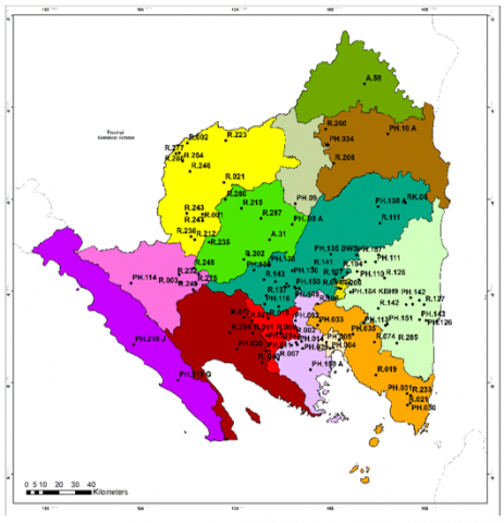
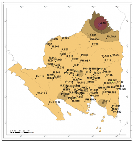
The method used in this research is descriptive quantitative. The research location is in Lampung Province, Indonesia. The data required consists of a map of Lampung Province and daily rainfall data from 126 manual rainfall measurement climatology stations and 4 automatic rainfall measurement climatology stations (Figure 1).
The research activities carried out consisted of collecting daily rainfall data and climatology stations measuring rainfall. Data were obtained in raw data in CSV format from each rainfall measurement station. It contains table information on rainfall events and the magnitude of each rain event. Second, perform a frequency analysis using the annual maximum data series to obtain statistical parameters with the type of distribution that meets the Smirnov-Kolmogorov test and the Chi-Square test [10]. Third, carry out an intensity analysis for a 10-year observation length (2011 – 2020) using daily rainfall data from a manual rainfall measurement climatology station in Lampung Province. Finally, the rainfall intensity is calculated using the Mononobe equation [11] and evaluate the relationship of variables between the IDF analysis originating from the climatology station for rainfall measurements and the IDF analysis originating from the climatology station.
Figure 1. Map of distribution of rainfall climatology stations in Lampung Province
2.1 Rainfall frequency analysis
Frequency analysis in hydrology determines the magnitude of the design rainfall and design flood with a certain return period. In practice, the major objective of the rainfall frequency analysis is to identify a suitable probability distribution to represent the connection between the magnitude and frequency of rainfall. The chosen distribution is fitted to a sample of observed rainfall data to enable extrapolation of the connection between the magnitude and frequency of rainfall outside the reported magnitudes and frequencies. However, it should be considered that such an extrapolation is always a guess: we will never know severe rainfall's "real" frequency. Frequency analysis can be done using data series obtained from historical rainfall data and discharge data. This study's rainfall data series used in the frequency analysis is the annual maximum series. Rainfall data is taken from the maximum rainfall data every year. The rainfall frequency distribution chosen in this study is a Log Pearson III distribution as reported by several research results [12-14].
2.2 Rainfall intensity analysis
Rainfall intensity is the height of rainwater per unit of time. The general nature of rainfall is that the shorter the rainfall, the intensity tends to be higher (vice versa). The relationship between the intensity, duration, and frequency of rainfall is usually expressed in the IDF curve. We need short-term rainfall data (60 minutes and 120 minutes) to get this. Rainfall data of this type can only be obtained from automatic rainfall measurement climatology stations. In addition, rainfall intensity can be calculated using the Mononobe equation if short-term rainfall data are unavailable. Calculating rainfall intensity can be utilized Mononobe formula as a representation in Equation 1 [11, 15].
$R_{t}=\frac{R_{24}}{24}\left(\frac{24}{T}\right)^{\frac{2}{3}}$ (1)
where, Rt is the rainfall intensity, R24 is maximum rainfall depth in a day, and T is duration of rainfall.
2.3 Relationship analysis
Relationship analysis is a form of research variable analysis to determine the strength of the relationship, the direction of the relationship between the variables, and the magnitude of the influence of the independent variable on the dependent variable. The approach used in analyzing this relationship includes correlation analysis which produces coefficients of determination and linear regression equations.
The coefficient of determination measures how far the model's ability to explain variations in the dependent variable (Equation 2). The value of the coefficient of determination is between zero and one. A small R² value means that the ability of the independent variable to explain the dependent variable is very limited. A close value means that the independent variable provides almost all the information needed to predict the dependent variable's variation simultaneously.
$R^{2}=1-\frac{\sum_{i=1}^{n}\left(A_{r}-F_{r}\right)^{2}}{\sum_{i=1}^{n}\left(A_{r}-A_{A}\right)^{2}}$ (2)
where, R2is coefficient of determination, n is number of fitted points, Ar is actual value of rainfall, Fr is forecast value of rainfall and AA is the average rainfall actual value.
2.4 Forecasting analysis of rainfall intensity
The purpose of forecasting is to produce an optimum forecast with no error or as little error as possible, which refers to a certain standard error. Therefore, every forecasting model must produce errors. If the resulting error rate is getting smaller, the forecasting results will be closer to the right. After all, stages are carried out, and the model is obtained, this model can then be used to forecast data for the next period. This research uses error analysis in Mean Absolute Percentage Error (MAPE). MAPE is a metric that indicates how accurate a forecasting system. It expresses this accuracy as a percentage and may be determined as the average absolute percent inaccuracy for each period divided by the actual values. To analyze MAPE used Equation 3. MAPE is one of the most frequently used tools for measuring the accuracy of forecasting models [16-18].
$M A P E=\frac{1}{n} \sum_{i=1}^{n}\left|\frac{A_{r}-F_{r}}{A_{r}}\right|$ (3)
where, MAPE is mean absolute percentage error, n is number of fitted points, Ar is actual value of rainfall, and Fr is forecast value of rainfall.
3.1 Calculation of frequency analysis
Daily rainfall data in this study is secondary data collected from 126 rainfall climatology stations spread over 15 districts and cities of Lampung Province. The research observation time is from 2011 to 2020. The selection of rainfall data used for frequency analysis uses a maximum series, which is done by taking one maximum data each year. A total of 126 rainfall climatology stations are available, there are 113 rainfall climatology stations with complete data for 10 years, and there are 13 rainfall climatology stations with incomplete data for 10 years. The incomplete rainfall climatology stations are presented in Table 1. The available data for each incomplete rainfall climatology station is 1 to 8 data out of 10 data that should be available. For the 13 stations with incomplete rainfall data for 10 years, distribution analysis using the Pearson III log was not followed up.
Table 1. Rainfall climatology stations with incomplete data for 10 years (2011-2020)
|
No. station |
Name of station |
Number of data rainfall |
|
39 |
PH.150A |
2 |
|
40 |
PH.149.A |
2 |
|
54 |
PH. 08.A |
1 |
|
60 |
PH.09 |
7 |
|
61 |
PH.10.A |
2 |
|
74 |
RK.06 |
7 |
|
85 |
PH.135 |
8 |
|
87 |
PH.138.A |
2 |
|
88 |
PH.138 |
8 |
|
94 |
PH.149 |
8 |
|
95 |
PH.150 |
8 |
|
115 |
PH.219 |
1 |
|
116 |
PH.218 |
1 |
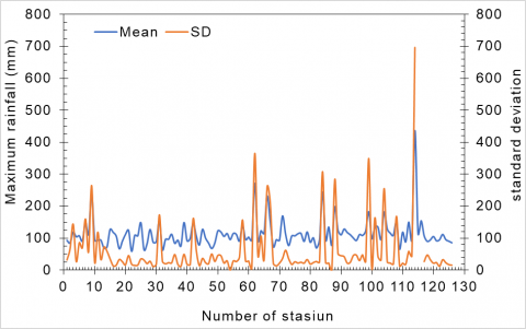
Frequency analysis is a procedure for estimating the frequency of an event in the future. This procedure can determine the design rainfall in various return periods based on the most suitable frequency distribution between the theoretical rainfall distribution and the empirical rainfall distribution. The average daily maximum rainfall data from 2011 to 2020 from 126 rainfall measurement climatological stations is presented in Figure 2. The distribution of the 126 climatological stations is shown in Figure 1. From Figure 2, it can be seen that the complete maximum daily rainfall data is available at 113 climatological stations from 126 climatological stations in this study.
By using the classification of rainfall from the Meteorology, Climatology, and Geophysics Agency (BMKG) Indonesia, there are 57 data from climatological stations, including the category with low rainfall (0 – 100 mm), 68 data from the climatology station, including the category with medium rainfall (100 – 300 mm), 1 data from the climatology station included in the category with high rainfall (300 – 500 mm). The average rainfall from 126 climatological stations is in the range of 58.3 – 435.6 mm. Furthermore, testing using the chi-square test method and the Smirnov Kolmogorov test on this rainfall distribution range is known that 5 stations cannot fulfill this test, namely station numbers 67 (R.284), 100 (R.141), 104 (R. 254), 111 (R.021), and 118 (PH.011).
Figure 2. Mean maximum rainfall (2011-2020) from 126 climatological stations in Lampung Province
3.2 Calculation of rain intensity
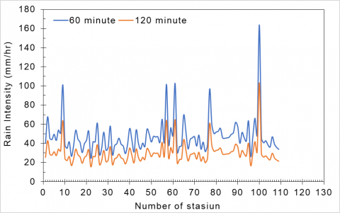
Rain intensity should be recorded in millimeters per hour (mm/hr). Mononobe equation can convert daily rainfall data into rain intensity data. Figure 3 The intensity of rain for a duration of 60 minutes is always greater than the duration of 120 minutes due to the time interval used to express the distribution of the amount of rain intensity. This duration was chosen for the drainage network design, and rain intensity data is needed when the rainfall intensity is high with a short duration.
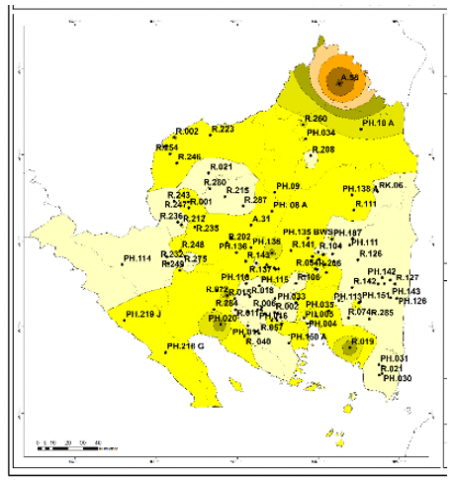
The analysis of rainfall intensity at 108 climatological rainfall stations in Lampung Province for a 5-year return period with 60 minutes and 120 minutes is included in the category of very heavy rainfall. This rainfall intensity data can be used in drainage design. The amount of rainfall intensity is then represented by making an isohyet map using ArcGIS, as shown in Figure 4 and Figure 5. This intensity map can then show the estimation of intensity values at climatological rainfall stations that do not meet the criteria for hydrological analysis. These results are in line with the research of Uzoigwe, et al. [19], who found that isohyet maps can be used to predict rainfall intensity in the ungauged basin in Nigeria.
Figure 3. Rainfall intensity from 109 rainfall climatology stations on a 5-year return period with a duration of 60 minutes in Lampung Province
Figure 4. Rainfall intensity map for 5-year return period 60 minutes duration
3.3 Analysis of the estimation of the intensity of the duration of the frequency using the rain intensity map method
Rainfall is the most important factor in the hydrological analysis. The planned rainfall event is the distribution of rain over time with selected characteristics. In general, the characteristics of the planned rainfall are the same as the characteristics of the rain that occurred in the past. If we can describe the characteristics of rainfall in a basin during hydrological analysis and planning, it is expected to describe rainfall events that occur in the future.
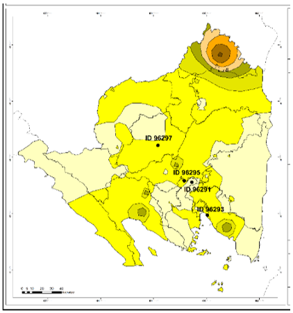
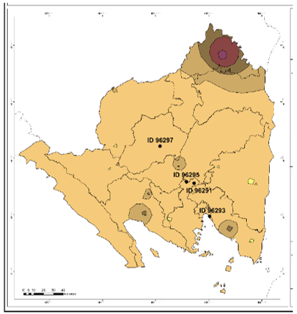
Often we find rainfall data that does not meet the criteria for hydrological analysis but is still used for hydrological analysis and planning for a basin. Analysis of the estimation of rainfall characteristics at rainfall climatology stations that do not meet the criteria of hydrological analysis can be obtained by the interpolation method using a rainfall intensity map from the surrounding rainfall climatology stations that meet the criteria of hydrological analysis. In addition to rainfall intensity maps for a 5-year return period with a short duration (Figure 4 and Figure 5), daily rainfall data from 4 complete climatological stations are also needed (Table 2).
Figure 5. Rainfall intensity map for 5-year return period 120 minutes duration
Table 2. Maximum daily rainfall from 4 climatological stations
|
Year |
Station 1 |
Station 2 |
Station 3 |
Station 4 |
|
2011 |
85 |
102 |
98 |
90.9 |
|
2012 |
129.4 |
82 |
95.2 |
70 |
|
2013 |
140 |
84.5 |
161 |
204.9 |
|
2014 |
108 |
68.5 |
102 |
110 |
|
2015 |
103 |
82.9 |
78.7 |
103.1 |
|
2016 |
109.5 |
135.5 |
96 |
112,4 |
|
2017 |
157 |
107 |
87.5 |
80.5 |
|
2018 |
137.5 |
100 |
115.5 |
81.4 |
|
2019 |
72 |
64 |
93 |
109.8 |
|
2020 |
103 |
119.5 |
89 |
115.3 |
|
Mean |
114.4 |
94.59 |
101.59 |
107.83 |
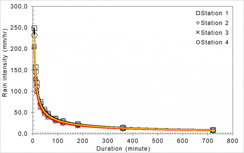
Furthermore, the frequency analysis of the rainfall data for the 4 complete climatological stations was carried out using the Pearson III Log distribution. The planned rainfall at various return periods following the Log Pearson Type III distribution at each climatological station was calculated using the chi-square and Smirnov Kolmogorov tests. Finally, rainfall intensity can be calculated using the Mononobe equation for a duration of 5 to 720 minutes over a 5-year return period (Figure 6). From Figure 6, a regression analysis was carried out to obtain the IDF curve and the Pearson correlation test value to see the close linear relationship between the independent variables (Eq. (4) to Eq. (7)). The results show that all correlation tests show a very strong relationship.
Ys1 = 726.1 ´ D-0.666 R2 = 1 (4)
Ys2 = 597.5 ´ D-0.666 R2 = 1 (5)
Ys3 = 600.8 ´ D-0.666 R2 = 1 (6)
Ys4 = 677.8 ´ D-0.666 R2 = 1 (7)
Figure 6. IDF curve of 5-year return period from 4 rainfall climatology stations
Rainfall intensity data from rainfall climatology stations that do not meet the hydrological criteria can be found by interpolating rainfall intensity maps from the nearest rainfall climatology station that meets the criteria for hydrological analysis. First, placed the coordinates of the location of the climatology station on the intensity map of the 5-year return period of 15, 30, 45, 60, 90, and 120 minutes, and then interpolating the rainfall intensity values at each climatology station based on the color on the map showing the intervals of rainfall intensity. The results are shown in Figure 7 and Figure 8 for a duration of 60 and 120 minutes, respectively.
The results of comparing the rainfall intensity from the Mononobe equation at 4 climatological stations with the rainfall intensity from the map interpolation at 4 climatological stations based on the intensity map are presented in Table 3. This Mean Absolute Percentage Error (MAPE) shows that the rainfall intensity with these two methods has good accuracy. This value indicates that the interpretation of rainfall with this approach can indicate that the rainfall intensity for climatological rainfall stations that do not meet the hydrological criteria can estimate the value of rainfall intensity derived from the isohyet intensity map from the climatological rainfall station in the vicinity that meets the requirements of hydrological analysis. This is in line with the results of research by Devianti et al. [20], who reported that mapping methods such as GIS could be used for various purposes, one of which is to estimate sedimentation in a watershed.In this study, GIS was employed for hydrological purposes in the form of prediction of bulk distribution. In contrast, in other studies, GIS was employed for hydrological purposes for sedimentation due to rainfall. However, this is a series of phenomena occurring in the hydrological sequence.
Table 3. Comparison of rainfall intensity values of the Mononobe approach with maps at 4 climatological stations
|
Stations |
Rainfall intensity (mm/hr) |
Error |
|||
|
Mononobe approach |
Isohyet approach |
||||
|
60 min |
120 min |
60 min |
120 min |
||
|
1 |
47.5 |
50 |
29.9 |
30 |
18.8 |
|
2 |
39.2 |
50 |
24.7 |
30 |
17.25 |
|
3 |
39.1 |
30 |
24.6 |
30 |
7.25 |
|
4 |
44.3 |
50 |
27.9 |
30 |
18.2 |
|
MAPE |
15.38 |
||||
Figure 7. Location of climatology station on map intensity of 5-year return period 60 minutes
Figure 8. Location of climatological stations on the map intensity of 5-year return period 120 minutes
IDF analysis for the ungauged basin with the method of determining the estimated rainfall intensity value based on the intensity map can be carried out. Rainfall intensity data from rainfall climatology stations that do not meet the hydrological criteria can be found by interpolating rainfall intensity maps from the nearest rainfall climatology station that meets the criteria for hydrological analysis. The value of the correlation analysis using MAPE was obtained at 15.38 (satisfactory). In addition, 45.24% of the rainfall data from the rainfall climatology station was included in the category of low rainfall, 53.97% of the rainfall data from the rainfall climatology station was included in the category of medium rainfall, and 0.79% of the rainfall data was from the climatology station. Rainfall is included in the category of high rainfall. The rainfall intensity value for the 5-year return period for 60 minutes and 120 minutes is categorized as very heavy rainfall. The interpretation of rainfall with the IDF approach can indicate that the intensity of rainfall for climatological rainfall stations that do not meet the hydrological criteria can still be estimated with the help of an isohyet intensity map from a nearby rainfall climatology station that meets the requirements of hydrological analysis.
[1] Markolf, S.A., Hoehne, C., Fraser, A., Chester, M.V., Underwood, B.S. (2019). Transportation resilience to climate change and extreme weather events – Beyond risk and robustness. Transport Policy, 74: 174-186. https://doi.org/10.1016/j.tranpol.2018.11.003
[2] Clark, S.S., Chester, M.V., Seager, T.P., Eisenberg, D.A. (2019). The vulnerability of interdependent urban infrastructure systems to climate change: could Phoenix experience a Katrina of extreme heat? Sustainable and Resilient Infrastructure, 4(1): 21-35. https://doi.org/10.1080/23789689.2018.1448668
[3] Payus, C., Ann Huey, L., Adnan, F., Besse Rimba, A., Mohan, G., Kumar Chapagain, S., Roder, G., Gasparatos, A., Fukushi, K. (2020). Impact of Extreme Drought Climate on Water Security in North Borneo: Case Study of Sabah. Water, 12(4): 1135.
[4] Mirhosseini, G., Srivastava, P., Stefanova, L. (2013). The impact of climate change on rainfall Intensity–Duration–Frequency (IDF) curves in Alabama. Regional Environmental Change, 13(1): 25-33. https://doi.org/10.1007/s10113-012-0375-5
[5] Fadhel, S., Rico-Ramirez, M.A., Han, D. (2017). Uncertainty of Intensity–Duration–Frequency (IDF) curves due to varied climate baseline periods. Journal of Hydrology, 547: 600-612. https://doi.org/10.1016/j.jhydrol.2017.02.013
[6] Mailhot, A., Duchesne, S., Caya, D., Talbot, G. (2007). Assessment of future change in intensity–duration–frequency (IDF) curves for Southern Quebec using the Canadian Regional Climate Model (CRCM). Journal of Hydrology, 347(1): 197-210. https://doi.org/10.1016/j.jhydrol.2007.09.019
[7] Dewi Sartika, T., Sihotang, R., Muslih, M., Sitorus, A., Haris, O., Bulan, R. (2020). Development of irrigation tank monitoring system and its environment for the effectiveness of rice irrigation. Acta Universitatis Agriculturae et Silviculturae Mendelianae Brunensis, 68(5): 859-865. https://doi.org/10.11118/actaun202068050859
[8] Al-Amri, N.S. Subyani, A.M. (2017). Generation of Rainfall Intensity Duration Frequency (IDF) Curves for Ungauged Sites in Arid Region. Earth Systems and Environment, 1(1): 8. https://doi.org/10.1007/s41748-017-0008-8
[9] El-Sayed, E.A.H. (2011). Generation of rainfall intensity duration frequency curves for ungauged sites. Nile Basin Water Sci Eng J, 4(1): 112-124.
[10] Moccia, B., Mineo, C., Ridolfi, E., Russo, F., Napolitano, F. (2021). Probability distributions of daily rainfall extremes in Lazio and Sicily, Italy, and design rainfall inferences. Journal of Hydrology: Regional Studies, 33: 100771. https://doi.org/10.1016/j.ejrh.2020.100771
[11] Kang, H., Shin, S., Paik, K. (2020). Power laws in intra-storm temporal rainfall variability. Journal of Hydrology, 590: 125233. https://doi.org/10.1016/j.jhydrol.2020.125233
[12] Devianti, Jayanti, D.S., Mulia, I., Sitorus, A., Sartika, T.D. (2019). Model of surface runoff estimation on oil palm plantation with or without biopore infiltration hole using SCS-CN and ANN methods. IOP Conference Series: Earth and Environmental Science, 365(1): 012065. https://doi.org/10.1088/1755-1315/365/1/012065
[13] Devianti, D., Bulan, R., Satriyo, P., Sartika, T.D. (2020). Study of hydroelectric power capacity using the rational method in the Lawe Sempali subwatershed, Aceh Province. Jurnal Pengelolaan Sumberdaya Alam dan Lingkungan (Journal of Natural Resources and Environmental Management), 10(2): 307-319. https://doi.org/10.29244/jpsl.10.2.307-319
[14] Juma, B., Olang, L.O., Hassan, M., Chasia, S., Bukachi, V., Shiundu, P., Mulligan, J. (2021). Analysis of rainfall extremes in the Ngong River Basin of Kenya: Towards integrated urban flood risk management. Physics and Chemistry of the Earth, Parts A/B/C, 124: 102929. https://doi.org/10.1016/j.pce.2020.102929
[15] Sartika, T.D., Pandjaitan, N.H., Sitorus, A. (2017). Measurement and modelling the drainage coefficient for hydraulic design criteria on residential area. in 3rd International Conference on Computing, Engineering, and Design, ICCED 2017, pp. 1-5. https://doi.org/10.1109/CED.2017.8308092
[16] Yin, H., Zheng, F., Duan, H.F., Savic, D., Kapelan, Z. (2022). Estimating rainfall intensity using an image-based deep learning model. Engineering. https://doi.org/10.1016/j.eng.2021.11.021
[17] Teixeira, D.B.D.S., Cecílio, R.A., Oliveira, J.P.B.D., Almeida, L.T.D., Pires, G.F. (2021). Rainfall erosivity and erosivity density through rainfall synthetic series for São Paulo State, Brazil: Assessment, regionalization and modeling. International Soil and Water Conservation Research. https://doi.org/10.1016/j.iswcr.2021.10.002
[18] Dankwa, P., Cudjoe, E., Amuah, E.E.Y., Kazapoe, R.W., Agyemang, E.P. (2021). Analyzing and forecasting rainfall patterns in the Manga-Bawku area, northeastern Ghana: Possible implication of climate change. Environmental Challenges, 5: 100354. https://doi.org/10.1016/j.envc.2021.100354
[19] Uzoigwe, L., Mbajiorgu, C., Alakwen, O. (2012). Development of intensity duration frequency (IDF) curve for parts of eastern catchments using modern ArcView GIS model. Special Publication of the Nigerian Association of Hydrological Sciences, 24-44.
[20] Devianti, Fachruddin, Purwati, Thamren, D.S., Sitorus, A. (2021). Application of geographic information systems and sediment routing methods in sediment mapping in Krueng Jreu Sub-Watershed, Aceh Province, Indonesia. International Journal of Sustainable Development and Planning, 16(7): 1253-1261. https://doi.org/10.18280/ijsdp.160706