Naveen Kumar Gavirineni | Edison Gundabattini*
© 2022 IIETA. This article is published by IIETA and is licensed under the CC BY 4.0 license (http://creativecommons.org/licenses/by/4.0/).
OPEN ACCESS
This paper analyzes the 660 MW supercritical thermal power plant design data, operation data, and various improvement strategies of all significant auxiliary equipment at various plant load factors. The effects of the plant load factor, auxiliary equipment performance and multiple properties of coal on equipment performance are discussed here. It is observed that the operation of the supercritical thermal power plant, at the maximum continuous rating, reduces the specific auxiliary power from 5.95% at 65% Plant load factor to 4.76% at 100% Plant load factor. Hence, there is a reduction in auxiliary power of total equipment by 68.80 MU/year. Also, due to the reduction of auxiliary power, CO2 emissions reduce to 65,300 tonnes, SO2 emission reduces to 4.752 tonnes, and NOx emission reduces to 2.898 tonnes. This paper discusses and analyzes the optimization of the process, optimization of excess air, improving energy efficiency measures for individual equipment, and controlling furnace ingress. Analysis indicates the increase in plant capacity and reduction in the auxiliary power by 0.8-1.2% of gross energy generation and also a release of an additional power 7.85 MW/hour to the concerned grid.
energy efficiency, plant load factor, coal consumption, flue gas, boiler feed water, excess air ratio, coal analysis, auxiliary power, CO2 emission
Thermal power plants are the measured sources of energy for the production of electrical power, and they generate different pollutants in the environment. Ecological effluence may be lessened by either minimizing the energy consumption or by generating high-efficient energy. In power plants some part of the energy being consumed by different auxiliary types of equipment. The auxiliary power is different for diverse plant sizes from 20 MW to 660 MW plants, varied between 13-4.75%. The Estimated auxiliary power used in 660 MW thermal power plants is 31.3 MW/hour; this generates CO2 emission by 751.2 t/d. Thermal power plant’s obtainability fundamentally depends on the availability of fuel, water facility, auxiliary systems, ash disposable stations, load dispatching centers and operation and maintenance reliability. There are so many reasons that auxiliary power consumption in India is higher than the other developed countries. Those are excessive feedwater flow, excessive steam flow, ineffective drives, deficiency of maintenance of apparatus, poor coal quality, internal leakage of equipment, lack of technology up-gradation, oversizing of equipment, and usage of unproductive control systems. Reduction in the auxiliary power by 0.5% may add 28.38 MU of additional power into the grid and 26,963 t/y CO2 emissions could be reduced.
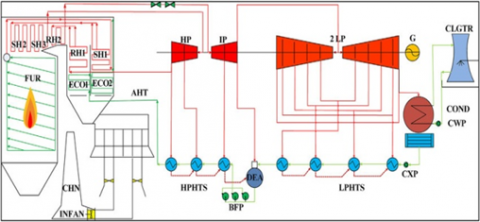
Supercritical once through units gives the maximum plant efficiency due to less losses from the boiler like unburnt carbon losses, dry flue gas losses, less moisture loss in combustion air and radiation losses and generates fewer pollutants than other subcritical and critical technology-based plants. Figure 1 shows the schematic of the 660 MW plant. In many countries, the vastly fluctuating grid frequency due to earthquake, physical attack, cyber attack, operations error, tsunamis, regional weather, ice storms, floods, space weather and other electromagnetic threats, hurricanes or tropical cyclones, wildfire, drought etc. This compels power units with superior part-load efficiency to realize greater economic power generation. Supercritical once through drum-less units are very useful for part load generation. Figure 2 shows the detailed process diagram and equipment.
1.1 Auxiliary power improvement
Bhatt and Mandi's [1] study indicated that the auxiliary power increases as gross energy generation (GEG) increase at full load conditions. They have identified the influencing parameters such as coal quality, excess steam flow, internal leakages, and inefficient drivers. Harley et al. [2] had studied bowl mills in pulverized coal boilers, at higher fineness (below 75 microns) power consumption of the mill is more and some carbon molecules escape from the furnace to increase carbon unburnt in fly ash. At low fineness (above 75 microns) power consumption of the mill is less than the designed values by adjusting rollers. Bhowmick and Bera [3] had studied the Induced draft performance, they had proved that Induced draft fan performance reduced due to over-design and older design (old electrostatic precipitator). Mandi et al. [4] studied the energy efficiency methods of boiler feed water pump in 210 MW thermal power plant. Their study indicated that the auxiliary power is reduced when the pump operated at 100% plant load factor. Also, the absence of re-circulation reduced the auxiliary power of the boiler feed water pump. Kumar and Rao [5] had studied the auxiliary power consumption of the total plant. Around 8% of energy generation from the plant was used to run the auxiliary equipment, and 30% for the boiler feed pump. Saha and Chatterjee [6] had compared the Indian auxiliary power consumption to other countries. They had concluded that Indian power generation units auxiliary power depletion are upper-sided due to low plant load factor, the higher ash content in coal, more steam flow, and feedwater flow consumption, lack of knowledge in the operation of utilities, design defects, etc. Adate and Awale [7] had studied boiler feed pump auxiliary power consumption and various factors affecting the auxiliary power consumption of boiler feed pump. They had concluded that the auxiliary power consumption of the feed pump could be decreased by enhancing the plant load factors. Raval and Patel [8] had studied different auxiliary power consumption and different improvement methods. They had studied in detail pumps and compressors, as these two are main auxiliaries that consume maximum power from the generation. Tsang [9] had experimented on impeller trimming (reduce the size of the impeller) of centrifugal pump. He had concluded that more trimming of impeller caused misalignment of impeller and casing. Chikkatur and Sagar [10] had done different studies about ash percentages in different coal, mill performance, and pollution generation. They concluded that 50% ash content in coal mill could increase power by 7.2% than the designed power.
1.2 Plant load factor improvement
Mandi and Yaragatti [11] had studied energy efficiency on 210 MW coal-fired power plants and concluded that the operation of the plant with improved PLF reduces the specific auxiliary power. Mandi and Yaragatti [12] had done energy-saving procedures in a 210 MW coal-fired power plant and concluded that the operation of the plant at enhanced PLF condensed the auxiliary power, net auxiliary power, and CO2 emission. CEA [13] had experimented on power plants with different plant load factors. Results indicated that by using supercritical and ultra-supercritical power plants, the plant load factor was improved and simultaneously specific auxiliary power was also decreased. Gomez [14] had studied rotary air preheater in a 210 MW coal-fired thermal power plant. He had done a detailed study in primary and secondary air heat extraction from flue gas. He had concluded that due to high pressure developed by PA and SA than flue gas, there was air leakage through APH that increased the gas flow and loading of ID fan. Sathyanathan and Mohammad [15] had studied the carbon percentage in both fly ash and bottom ash. They had found that fly ash combustibles depend on proximate analysis and GCV of coal, whereas bottom ash combustibles depend on coal particle size (50 mesh particles).
Figure 1. Line diagram of 660 MW Supercritical thermal power plant [1]
Figure 2. A 660 MW supercritical power plant schematic representation [16]
1.3 Optimization of pollution levels
Krol and Oclon [17] had studied the performance improvement prices and CO2 emission prices. They concluded that CO2 emission and fuel cost had a strong influence when coal handling plants connect with condensing turbines at low pressure. Javadi et al. [18] experimented on a 500 MW combined cycle power plant for the optimization of CO2 emission, system exergy efficiency, and energy cost to reduce the heat rate. Manzolinia et al. [19] had worked in the STEPWISE H2020 project and the SEWGS technology integrated with Iron and steel plant to know CO2 emission levels. They concluded that the SEWGS technology has enhanced steam consumption that increases energy. Kumar et al. [20] had studied coal thermal power plants in terms of emission taxation and used linear programming-based data envelopment analysis (DEA) to estimate boiler efficiency. Chen [21] had examined the changes in productivity from the regulations of the environment to control the CO2 emission in thermal power plants. They concluded that measuring productivity advancement by shadow pricing is more than the actual trading price of CO2. Liu et al. [22] had studied different environmental and pollutions issues from thermal power plants in China, they have concluded that in China thermal power plants releasing greater emissions than other sectors. Lysko et al. [23] had analysed the various emissions generations, equipment-wise auxiliary power consumption, station auxiliary power consumption, operation reliability. They had proved that CO2 emission production is equivalent to coal consumption in the plant.
1.4 Energy efficiency improvements
Mahmoudi et al. [24] had identified approaches such as multivariate data analysis to improve the boiler performance and to decrease different emissions relating rate to the atmosphere. Joskow and Schmalensee [25] had analysed the thermal efficiency and consistency of electric generating units with coal burning, they had concluded that an increase in the steam pressure of generating units had led to advances in thermal efficiency. Kumar and Rao [26] had listed the various parameters like coal flow, feedwater flow, steam flow, airflow, excess air ratios, boiler, and turbine operation. They concluded that heat loss due to hydrogen is more than other heat losses. Franco and Casarosa [27] had explored the possibilities to increase the combined cycle plant efficiency. Results indicated that the hot reheat steam generator achieves 60% by using regenerator turbine exhaust gas temperature. Mandi et al. [28, 29] had studied the air-cooled and water-cooled condenser and cooling tower in a water-cooled condenser. They had concluded that with the less cooling tower makeup water the heat exchanger capacity of the condenser could be increased. Srinivas [30] had studied the dual pressure heat recovery steam generator (HRSG). He has concluded that optimization of combustion system possible at a temperature of 1400℃ with turbine blade cooling technology.
In this paper, we have analyzed a 660 MW supercritical thermal power plant considering various parameters viz. different plant load factors, different coal properties, and improving energy efficiency measures for equipment. We have also analyzed various methods to improve auxiliary power improvement of individual equipment like various boiler losses; excess air optimization techniques on different coal samples consequently studied the coal consumption and different emission levels generation from the plant.
The plant load factor is the ratio of average load generation to the peak load in a particular period. This is the degree of the output of a power plant in comparison to the maximum output [5]. Some of the power plants are operating their load at a low plant load factor that causes high auxiliary power consumption, increase coal consumption, and emissions. There is a close relationship between plant load factor and generated output, and these two are directly proportional to both Boiler output and turbine output. Boiler output i.e., steam generation depends on airflow, flue gas flow, coal flow, feedwater flow, condensate flow [18], and pressure gain across fans and pumps. Similarly, turbine output i.e., power generation depends on condenser vacuum, steam pressure, steam flow, and steam enthalpy. Power consumption on individual drives depends on equipment running load if the equipment running at full load specific auxiliary power reduces [20].
Lower PLF lessens the generation of power and also reduces the feedwater flow, condensate flow, air flows, and flue gas flow. Lower plant load factors are also due to specific steam consumption (ratio between steam flows in t/h to GEG in MW), specific fuel consumption (ratio between fuel consumption in t/h to GEG in MW), and specific energy consumption (ratio between electrical power consumption in MW to the feed/condensate water consumption in tones). The equation of variation in fluid flow in second-order polynomial with plant load factor:
Fluid flow $=\mathrm{A}_{0}+\mathrm{A}_{1} * \mathrm{PLF}+\mathrm{A}_{2} * \mathrm{PLF}^{2} \mathrm{t} / \mathrm{h}$
The deviation of fluid flow with different PLF’S given in Figures 3-7. Let A0, A1, A2 are coefficients, and standard deviation R2, Table 1. The stable levels of various flows are more than 99% as shown by the Polynomial second-order curve-fit.
Figure 3 shows the comparison of operating feed water flows with design feedwater flow, at 100% PLF as per the supplier recommendation 1771 t/h but in the actual feed, water flows consumption of boiler 1810 t/h. This is due to the loss of steam to the atmosphere through safety valve passing, steam purge valve passing, heater drains passing, etc. The deviation of feedwater flow range of 3-40 t/h.
Table 1. Different fluid flows fit curve values with PLF (50-100%) at 660 MW plant
|
S.NO |
Equipment |
X-axis |
Y-axis |
Constant(A0) |
Constant(A1) |
Constant(A2) |
Standard, R2 |
|
1 |
ID Fans |
PLF's |
Flue Gas Flows |
679.106 |
-4.151 |
0.176 |
0.984 |
|
2 |
FD Fans |
PLF's |
Secondary Air Flows |
450.309 |
17.240 |
-0.011 |
0.987 |
|
3 |
PA Fans |
PLF's |
Primary Air Flows |
292.388 |
-2.468 |
0.044 |
0.989 |
|
4 |
Mills |
PLF's |
Coal Flow |
-6.774 |
4.415 |
-0.002 |
0.968 |
|
5 |
BFP |
PLF's |
Feed Water Flow |
416.236 |
15.928 |
0.021 |
0.996 |
|
6 |
CEP |
PLF's |
Condensate Water Flow |
-0.272 |
0.011 |
0.003 |
0.995 |
Figure 3. Comparison of Design VS Operating feed water flows at different PLF’S
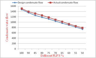
Figure 4. Comparison of Design VS Operating condensed water flows at different PLF’S
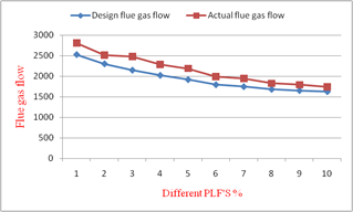
Figure 5. Comparison of Design VS Actual flue gas flows at different PLF'S
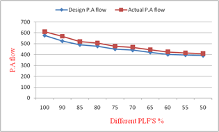
Figure 6. Comparison of Design VS Operating Primary Air flows at different PLF’S
Figure 4 shows the comparison of operating condensate water flow with design condensate water flow, at 100% PLF as per the supplier recommendation 1474 t/h whereas the condensed water flow consumption of boiler is 1512.37 t/h. This is due to the loss of steam to the atmosphere through the LP heater drain passage. The deviation of feedwater flow is in the range of 38-70 t/h.
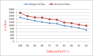
Figure 5 shows the comparison of actual flue gas flow with design flue gas flow. Flue gas flow at 100% PLF, as per the supplier recommendation, is 2524.5 t/h whereas the actual flue gas flow from the boiler is 2810 t/h. This is due to the loss of flue gas through ducting system and loss through the rotary air preheater.
Figure 6 shows the comparison of actual PA flow with design PA flow; at 100% PLF as per the supplier recommendation design PA flow is 576.77 t/h whereas the actual PA flow supplies to the boiler are 610.2t/h. This is due to the loss of air through the rotary air preheater.
Figure 7 shows the comparison of actual SA flow with design SA flow, at 100% PLF as per the supplier recommendation design SA flow is 1501.4 t/h whereas the actual SA flow supplies to the boiler 1782.8 t/h. This is due to the loss of air through the rotary air preheater.
Figure 7. Comparison of Design VS Operating Secondary Air flows at different PLF’S
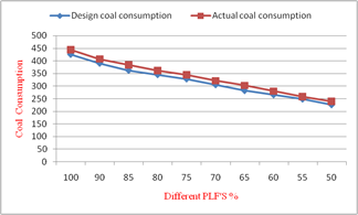
Figure 8. Comparison of Design VS Operating Coal flows at different PLF’S
Figure 8 shows the comparison of actual coal flow with design coal flow, at 100% PLF as per the supplier recommendation design coal flow is 425 t/h whereas the actual coal flow supplies to the boiler 445 t/h. This is due to the loss of boiler performance and increase of turbine heat rate.
2.1 Deviation in fluid flow
Fluid flow varies according to different loads. The boiler manufacturer provides values of the fluid flow for different loads (design data), but in running conditions, there may be a deviation from the design conditions of the plant.
Deviation in fluid flow $\frac{\left(m_{\mathrm{r}}-m_{\mathrm{o}}\right) * 100 \%}{\left(m_{\mathrm{r}}\right)}$
where, mr= Fluid flow operation from BFP, Primary airflow from PA fans, Condensate flow from CEP, Secondary airflow from FD fans, Coal flow from mills, flue gas flow from ID fans; operating = At full load 660 MWexact Fluid flow from BFP, Primary airflow from PA fans, Condensate flow from CEP, Secondary airflow from FD fans, Coal flow from mills, flue gas flow from ID fans.
In a 660 MW power plant under full load conditions, the deviation of fluid flows is polynomial curve-fitted in the second-order derivative, Figure 9. From the deviation of fluid flows data (curve-fitted in second-order derivations), three constants and standard deviation could be found out.
Deviation in Fluid flow $=\mathrm{B}_{\mathrm{o}}+\mathrm{B}_{1} * \mathrm{PLF}+\mathrm{B}_{2} * \mathrm{PLF}^{2} \%$
where, B0, B1, B2 coefficients, and R2 standard deviation for all major equipment. The curve-fit second-order polynomial of variation of different flows given in Table 2. The values are in the range of 0.868 – 0.968. The value of the curve-fit for flue gas flow is 0.868, primary airflow is 0.968, secondary airflow is 0.953, coal flow is 0.957, feedwater flow is 0.926, and condensate flow is 0.948.
Figure 9. Deviation of different fluid flows with PLF (50-100%) at 660 MW plant
Table 2. Deviation of different fluid flows curve-fit values with PLF (50-100%) at 660 MW plant
|
S.NO |
Equipment |
X-axis |
Y-axis |
Constant(B0) |
Constant(B1) |
Constant(B2) |
Standard, R2 |
|
1 |
I.D Fans |
PLF's |
Flue Gas Flows |
-123.910 |
16.968 |
-0.090 |
0.868 |
|
2 |
F.D Fans |
PLF's |
Secondary Air Flows |
62.124 |
-6.759 |
0.048 |
0.953 |
|
3 |
P.A Fans |
PLF's |
Primary Air Flows |
-91.444 |
0.807 |
-0.003 |
0.968 |
|
4 |
Mills |
PLF's |
Coal Flow |
-63.975 |
0.707 |
-0.004 |
0.957 |
|
5 |
B.F.P |
PLF's |
Feed Water Flow |
-138.078 |
3.340 |
-0.027 |
0.926 |
|
6 |
C.E.P |
PLF's |
Condensate Water Flow |
41.722 |
5.278 |
-0.035 |
0.948 |
Following components and factors affect the plant load factor:
The initial starting of the plant requires power and is supplied by external grids on a chargeable basis. The power could be distributed to equipment by station transformer which is located adjacent to the GT. Once power generation starts, power is available for running the equipment, this power is called unit auxiliary power. This power is tapped from the unit auxiliary transformer. The unit auxiliary power transformer supplies power to all equipment. The auxiliary power could be divided into two groups, in-house auxiliary power and Out-door auxiliary power or general auxiliary power.
The In-house auxiliary power equipment: Forced draft fans (FD), Boiler feed pumps (BFP), Primary air fans (PA), Induced draft fans (ID), Coal mills (pulverizes), and Condensate extraction pumps (CEP). Out-door or general auxiliary power is the power used for general tools such as auxiliary cooling water pumps (ACW), Circulating water pumps (CW), Demineralised water pumps, ash water pumps, Conveyors, Belts, Crushers, Common lighting available in the plant. Table 3 shows the major auxiliary power details.
Some power is always needed for the running of equipment; hence the specific power is defined as the ratio of power consumed by the equipment at motor terminals to the maximum generation.
SpecificAuxiliarypower $=\frac{(\mathrm{Pm} * 100)}{(\mathrm{Pl} * 100)}$
where, Pm = Measured power input to the motor, Pl= Measured P.L.F.
The specific auxiliary power of HT equipment is polynomial curve-fitted and is second-order concerning PLF.
Auxiliary Power (A.P) = 8.9*10-5 *PLF2-0.098162*PLF + 17.66993%
Table 4 shows the standard deviation for the second-order polynomial curve-fit is 0.978. It is showing a confidence level is more than 97%. It is appropriate and the scatter of data for the given units is within 2-3%.
Deviation in Auxiliary power $=\mathrm{C}_{0}+\mathrm{C}_{1} * \mathrm{PLF}+\mathrm{C}_{2} * \mathrm{PLF}^{2} \%$
where, C0, C 1, C 2 coefficients and R2 standard deviation given for all major equipment. The curve-fit second-order polynomial of variation of different specific auxiliary power is given in Table 4.
Deviation in Auxiliary power at various PLF’s in 660 MW.
unit $=\frac{\left(A P_{\mathrm{r}}-A P_{\mathrm{o}}\right) * 100 \%}{\left(A P_{\mathrm{r}}\right)}$
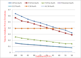
where, APr is the rated/design auxiliary power in kW, APo is the present operating auxiliary power in kW. The polynomial curve-fit for various specific auxiliary power with different PLF’s is in the range of 0.88-0.99% shown in Table 5. The attainable efficiency level of ID Fan is 88.07%, but in reality, it is low due to air leakage through APH, air enters through ducts, and hydrodynamic pressure drop.
In a 660 MW power plant under full load conditions, the deviation in different auxiliary power consumption and the deviation in auxiliary power is polynomial curve-fitted in the second-order derivative, Figure 10. From the deviation in auxiliary power consumption data (curve-fitted in second-order derivations), three constants and standard deviation could be found out.
Deviation in Auxiliary power of equipment $=\mathrm{D}_{\mathrm{o}}+\mathrm{D}_{1} * \mathrm{PLF}+\mathrm{D}_{2} * \mathrm{PLF}^{2} \%$
where, D0, D 1, D 2 coefficients, and R2 standard deviation given for all the major equipment. The curve-fitted second-order polynomial of variation of different specific auxiliary power is given in Table 6.
Figure 10. Deviation of different equipment auxiliary power consumption with PLF (50-100%) at 660 MW plant
Table 3. Details about the primary auxiliary power equipment (in-house)
|
S.No |
Equipment |
No. of equipment (Running/ Standby) |
Equipment Description |
Speed, rpm |
Efficiency, % |
Motor Rating, kW |
Fluid flow |
|
1 |
ID Fan |
2+0 |
Axial Reaction with Variable Blade pitch control |
745 |
84.5 |
4200 |
710 |
|
2 |
FD Fan |
2+0 |
Axial Reaction with Variable Blade pitch control |
990 |
84.5 |
1700 |
280 |
|
3 |
PA Fan |
2+0 |
Axial Reaction with Variable Blade pitch control |
1490 |
87.5 |
3750 |
220 |
|
4 |
Pulverizer |
5+1 |
Bowl mill |
989 |
82.5 |
1000 |
85 |
|
5 |
BFP |
2+1 |
Horizontal, centrifugal type with barrel casing |
2900 |
85.7 |
10859 |
1439.8 |
|
6 |
CEP |
1+1 |
Vertical, multistage |
1480 |
94 |
1040 |
849 |
|
7 |
CW Pumps |
2+1 |
Vertical, self-water cooling |
330 |
89.78 |
2600 |
29330 |
|
8 |
ACW Pump |
2+1 |
Horizontal, centrifugal, multistage |
983 |
86.25 |
110 |
2275 |
Table 4. Different auxiliary power curve-fit values with PLF (50-100%) at 660 MW plant
|
S.NO |
Equipment |
X-axis |
Y-axis |
Constant1 |
Constant2 |
Constant3 |
Standard, R2 |
|
1 |
Auxiliary power Design |
PLF's |
Auxiliary power in MW |
8.6325 |
-0.10337 |
0.0004 |
0.98513 |
|
2 |
Auxiliary power Operation |
PLF's |
Auxiliary power in MW |
8.81244 |
-0.09289 |
0.00035 |
0.97863 |
Table 5. Different auxiliary power values at different P.L.F
|
S.No |
Equipment |
X-axis |
Y-axis |
Constant (C0) |
Constant (C1) |
Constant (C2) |
Standard R2 |
|
1 |
ID Fans |
PLF's |
ID Fan Power Consumption |
0.6241 |
0.0303 |
-0.0001 |
0.8807 |
|
2 |
FD Fans |
PLF's |
FD Fan Power Consumption |
0.7038 |
-0.0014 |
0.0001 |
0.9798 |
|
3 |
PA Fans |
PLF's |
PA Fan Power Consumption |
0.5738 |
0.0178 |
0.0000 |
0.9856 |
|
4 |
Mills |
PLF's |
Mill Fan Power Consumption |
0.0080 |
0.0065 |
0.0000 |
0.9754 |
|
5 |
CEP |
PLF's |
CEP Fan Power Consumption |
0.0958 |
0.0112 |
0.0000 |
0.9947 |
Table 6. Deviation of different auxiliary power curve-fit values with PLF (50-100%) at 660 MW plant
|
S.NO |
Equipment |
X-axis |
Y-axis |
Constant(D0) |
Constant(D1) |
Constant(D2) |
Standard, R2 |
|
1 |
ID Fans |
PLF's |
I.D Fan Power Consumption |
-0.734 |
0.015 |
0.003 |
0.975 |
|
2 |
FD Fans |
PLF's |
F.D Fan Power Consumption |
-0.744 |
0.022 |
0.003 |
0.976 |
|
3 |
PA Fans |
PLF's |
P.A Fan Power Consumption |
-0.878 |
0.034 |
0.008 |
0.996 |
|
4 |
Mills |
PLF's |
Mill Fan Power Consumption |
-0.046 |
0.005 |
0.002 |
0.999 |
|
5 |
CEP |
PLF's |
C.E.P Fan Power Consumption |
0.261 |
0.000 |
0.009 |
0.865 |
Table 7. Different specific energy consumption values at different PLF
|
S.NO |
Equipment |
X-axis |
Y-axis |
Constant(E0) |
Constant(E1) |
Constant(E2) |
Standard, R2 |
|
1 |
ID Fans |
PLF's |
SEC of ID fans |
0.5459 |
-0.05823 |
0.000852 |
0.728 |
|
2 |
FD Fans |
PLF's |
SEC of FD fans |
0.6264 |
-0.0821 |
0.000628 |
0.952 |
|
3 |
PA Fans |
PLF's |
SEC of PA fans |
0.7682 |
-0.2258 |
0.000232 |
0.982 |
|
4 |
Mills |
PLF's |
SEC of Mills |
1.2568 |
-0.1235 |
-0.000982 |
0.956 |
|
5 |
CEP |
PLF's |
SEC of CEP |
0.6282 |
-0.2185 |
0.000462 |
0.889 |
The specific energy consumption for individual equipment as:
Specific energy consumption $=\frac{\text { Equipment power }}{\text { Feedwaterflow }} \mathrm{KW} /$ ton
The changes of specific energy consumption of all equipment are a second-order polynomial with different PLF’s:
Specific energy consumption $=\mathrm{E}_{\mathrm{o}}+\mathrm{E}_{1} * \mathrm{PLF}+\mathrm{E}_{2} * \mathrm{PLF}^{2} \%$
where, E0, E 1and E2 are coefficients and R2 is the standard deviation for all HT auxiliary equipment, Table 7.
The polynomial curve-fit values of standard deviation are in the range 0.728-0.982. The achievable efficiency levels for ID fan are 72.8%, for CEP is 88.9%, for FD fan is 95.2%, for Mill is 95.6%, etc. But in reality, the values are less due to incombustible air enters through APH and ducts which do not take part in the combustion. This air reduces the capacity of the ID fan.
The performance test was conducted on 2 units of 660 MW units. Two units were having a common station transformer where the station loads were distributed and having the same equipment such as ID Fans, BFP, PA Fans, FD Fans, and CEP, etc. Performance tests were conducted on Boiler and Turbine from PTC 4.1 and PTC 6.1. Blended coal having a 70:30 proportion was used as an input to the Boiler. The test was conducted for nearly 3 hours on full load. During the test period, the blowdown, soot blowing, and equipment changeover were halted to obtain an accurate result.
3.1 Detailed study on the HT- In-house auxiliary equipment
4.1 Component parameters to improve the plant load factor of 660 MW thermal power plant
The PLF improvement mainly depends on the capacity of all HT auxiliary equipment like ID fan, FD fan, PA fan, BFP, CEP, etc. There are few improvement methods to increase the performance of HT auxiliary equipment for increasing the plant load factor of 660 MW supercritical thermal power plants. Some of the methods are discussed here.
4.2 Induced draft fans
ID fan performance could be improved by improving the following factors listed here:
a) I.D fan capacity increases by reducing flue gas flow, this depends on the calorific value and ash content of coal. Always low ash content and higher calorific value of coal are preferable for 660 MW units. Here consider four different coal samples with different coal proportions which are shown in Table 8. Ash in the coal reduces from 44.3% in case I to 32.1% in case IV, increase boiler efficiency from 83.93% to 86.14% [31] could reduce auxiliary power from 1000 kWh to 868.2 kWh and reduced the total auxiliary power by 0.11%. ID fan efficiency increased from 48.65% to 53.5% and reduce coal consumption to 0.5 tones. The expected average reduction in CO2 emission is 0.475 tones.
b) ID fan capacity increases by improving the efficiency of ESP from 92.5% to 98.8% by injecting NH3 into the flue gas and decreasing the erosion rate of the ID fan impeller as well.
Table 8. Various losses in Boiler according to various coal samples
|
660 MW |
660 MW |
660 MW |
660 MW |
|||
|
S.No |
Description |
Unit |
Sample1 |
Sample2 |
Sample3 |
Sample4 |
|
|
Proximate analysis |
|||||
|
|
Fixed Carbon |
% |
17.3 |
26.4 |
20.1 |
23.28 |
|
|
Ash |
% |
44.3 |
26.65 |
39.7 |
32.0 |
|
|
Volatile Matter |
% |
19.0 |
23.6 |
20.0 |
22.0 |
|
|
Moisture- Inherent |
% |
19.4 |
23.35 |
20.2 |
22.72 |
|
|
Gross Calorific Value - A.R.B |
Kcal/Kg |
3630.52 |
3856.68 |
3700.82 |
3820.0 |
|
|
Boiler efficiency by heat loss method |
|||||
|
I |
Unburnt carbon losses |
% |
3.040 |
1.722 |
2.791 |
1.706 |
|
II |
Fly ash caused sensible heat loss |
% |
0.251 |
0.134 |
0.207 |
0.155 |
|
III |
Bed ash caused Sensible heat loss |
% |
0.492 |
0.279 |
0.436 |
0.335 |
|
IV |
Moisture in combustion air caused loss |
% |
0.061 |
0.066 |
0.056 |
0.056 |
|
V |
Moisture in fuel caused loss |
% |
3.385 |
3.819 |
3.441 |
3.738 |
|
VI |
Hydrogen in fuel caused loss |
% |
4.382 |
4.166 |
4.446 |
4.146 |
|
VII |
Dry flue gas caused loss |
% |
4.200 |
4.216 |
3.793 |
3.450 |
|
VII |
Radiation loss |
% |
0.250 |
0.250 |
0.250 |
0.250 |
|
|
Boiler efficiency |
83.939 |
85.347 |
84.580 |
86.164 |
|
4.3 Boiler feed pump (BFP)
Boiler feed pump performance would be improved by the following factors as discussed,
4.4 Mills/Pulverizers
Mill performance was improved by the following factors as discussed herewith
4.5 Condensate extraction pump (C.E.P)
Condensate extraction pump performance was improved by the following factors:
4.6 Forced draft fans (FD)
Forced draft fans performance was improved by the following factors as discussed herewith:
4.7 Primary air fans (PA)
Primary air fans performance was improved by the following factors as discussed herewith:
Power plant operating at 60-100% maximum continuous rating condition, could reduce auxiliary power consumption from 5.95% to 4.76% in a 660 MW supercritical thermal power plant. At this 60-100% maximum continuous rating condition, the auxiliary power is reduced by 68.80 MU/year causing the reduction of CO2 emissions by 65,300 t/y. After optimizing the excess air and selection of low ash coal save power consumption by 97 kW/hour which is an equivalent reduction of CO2 by 0.1018 t/y and overhauling of plant equipment reduces hydrodynamic resistance of flue gas which reduces the auxiliary power by 0.11% of gross energy generation. By maintaining the performance of individual equipment, optimum excess air, and controlling furnace ingress through proper maintenance, the auxiliary power is reduced by 1.05% of gross energy. The overall reduction of auxiliary power from various methods could be 1.19% i.e., equivalent to a CO2 reduction of 65,300 t/y and added surplus power of 7.85 MW/hour into the grid through the energy conservation techniques.
We appreciate the work and technical data support by M/s. Lalitpur Power Generation Company Limited. The authors are deeply thankful to all the technical and non-technical staff members for their cooperation and kind support in conducting the experiments.
|
Abbreviations |
|
|
CO2 |
Carbon dioxide |
|
SOX |
Sulphur oxide |
|
NOX |
Nitrogen oxide |
|
SO2 |
Sulfur dioxide |
|
MW |
Mega Watt |
|
PLF |
Plant load factor |
|
ID |
Induced draft |
|
FD |
Forced draft |
|
MU |
Million Units |
|
SO2 |
Sulfur dioxide |
|
GCV |
Gross calorific value |
|
APH |
Air preheater |
|
PA |
Primary air |
|
SA |
Secondary air |
|
ESP |
Electro static precipitator |
|
BFP |
Boiler feed pump |
|
CEP |
Condensate extraction pump |
|
HP |
High pressure |
|
LP |
Low pressure |
|
CHP |
Coal handling plant |
|
PTC |
Power trading corporation |
|
NH3 |
Ammonia |
|
IGV |
Internal guided vanes |
|
VFD |
Variable frequency drive |
|
HT |
High tension |
|
LT |
Low tension |
|
GEC |
Gross Energy Generation |
|
SEWGS |
Sorption Enhanced Water Gas |
|
Acronyms |
|
|
% |
Percentage |
|
R2 |
Standard deviation |
|
Pm |
Measured power |
|
℃ |
Degree Centigrade |
|
kWh |
Kilowatt-hour |
|
mmwc |
millimeter of the water column |
|
t |
tones |
|
t/h |
tones per hour |
|
kW |
kilowatt |
|
k-Cal/kg |
kilocalories per kilogram |
|
kPa |
kilo Pascals |
|
$m_{\mathrm{r}}$ |
rated mass |
|
$m_{\mathrm{o}}$ |
operating mass |
|
t/y |
tones per year |
|
t/d |
tones per day |
[1] Bhatt, M.S., Mandi, R.P. (1999). Performance enhancement in coal‐fired thermal power plants. Part III: auxiliary power. International Journal of Energy Research, 23(9): 779-804. https://doi.org/10.1002/(SICI)1099-114X(199907)23:9<779::AID-ER514>3.0.CO;2-P
[2] Harley, C., Trunkett, K.S. (2003). Coal-Gen-Improving Plant Performance with Advanced Wear Protection Technologies. Conforma Clad Inc., Albany.
[3] Bhowmick, M.S., Bera, S.C. (2008). Study the Performances of induced fans and design of new induced fan for the efficiency improvement of a thermal power plant. In 2008 IEEE Region 10 and the Third international Conference on Industrial and Information Systems, pp. 1-5. https://doi.org/10.1109/ICIINFS.2008.4798468
[4] Mandi, R.P., Seetharamu, S., Yaragatti, U.R. (2014). Enhancing energy efficiency of boiler feed pumps in thermal power plants through operational optimization and energy conservation. International Research Journal of Power and Energy Engineering, 1(1): 2-11.
[5] Kumar, C.K., Rao, G.S. (2013). Performance analysis from the energy audit of a thermal power plant. International Journal of Engineering trends and Technology (IJETT), 4(6): 2488-2490.
[6] Saha, A., Chatterjee, S. (2005). Achievements in thermal and electrical energy conservation at budge budge generating station, CSES limited. In Proceedings of National workshop on Energy Conservation for Power Engineers, at PMC, Noida, New Delhi, Organized by NTPC, pp. 32-42.
[7] Adate, N.D., Awale, R.N. (2013). Energy conservation through energy efficient technologies at thermal power plant. International Journal of Power System Operation and Energy Management, ISSN (PRINT), 2231-4407.
[8] Raval, T.N., Patel, R.N. (2013). Optimization of auxiliary power consumption of combined cycle power plant. Procedia Engineering, 51: 751-757. https://doi.org/10.1016/j.proeng.2013.01.107
[9] Tsang, L.M. (1992). A theoretical account of impeller trimming of the centrifugal pump. Proceedings of the Institution of Mechanical Engineers, Part C: Journal of Mechanical Engineering Science, 206(3): 213-214. https://doi.org/10.1243/PIME_PROC_1992_206_117_02
[10] Chikkatur, A.P., Sagar, A.D. (2007). Cleaner power in India: Towards a clean-coal-technology roadmap. Belfer Center for Science and International Affairs Discussion Paper, 6: 1-261.
[11] Mandi, R.P., Yaragatti, U.R. (2014). Control of CO2 emission through enhancing energy efficiency of auxiliary power equipment in thermal power plant. International Journal of Electrical Power & Energy Systems, 62: 744-752. https://doi.org/10.1016/j.ijepes.2014.05.039
[12] Mandi, R.P., Yaragatti, U.R. (2012). Energy efficiency improvement of auxiliary power equipment in thermal power plant through operational optimization. In 2012 IEEE International Conference on Power Electronics, Drives and Energy Systems (PEDES), pp. 1-8. https://doi.org/10.1109/PEDES.2012.6484459
[13] Performance Review of Thermal Power Stations 1999–00, 2006–07, 2007–2008, 2008–09, 2009–10, 2010–11, and 2011–12. Website: <http://www.cea.nic.in>.
[14] Gomez, J.L. (1987). Modeling of air leakages on a Tri-sector Air heater. Public Service Indiana.
[15] Sathyanathan, V.T., Mohammad, K.P. (2004). Prediction of unburnt carbon in tangentially fired boiler using Indian coals. Fuel, 83(16): 2217-2227. https://doi.org/10.1016/j.fuel.2004.05.004
[16] Adibhatla, S., Kaushik, S.C. (2014). Energy and exergy analysis of a super critical thermal power plant at various load conditions under constant and pure sliding pressure operation. Applied Thermal Engineering, 73(1): 51-65. https://doi.org/10.1016/j.applthermaleng.2014.07.030
[17] Król, J., Ocłoń, P. (2019). Sensitivity analysis of hybrid combined heat and power plant on fuel and CO2 emission allowances price change. Energy Conversion and Management, 196: 127-148. https://doi.org/10.1016/j.enconman.2019.05.090
[18] Javadi, M.A., Hoseinzadeh, S., Khalaji, M., Ghasemiasl, R. (2019). Optimization and analysis of exergy, economic, and environmental of a combined cycle power plant. Sādhanā, 44(5): 1-11. https://doi.org/10.1007/s12046-019-1102-4
[19] Manzolini, G., Giuffrida, A., Cobden, P.D., van Dijk, H.A.J., Ruggeri, F., Consonni, F. (2020). Techno-economic assessment of SEWGS technology when applied to integrated steel-plant for CO2 emission mitigation. International Journal of Greenhouse Gas Control, 94: 102935. https://doi.org/10.1016/j.ijggc.2019.102935
[20] Kumar, S., Managi, S., Jain, R.K. (2020). CO2 mitigation policy for Indian thermal power sector: Potential gains from emission trading. Energy Economics, 86: 104653. https://doi.org/10.1016/j.eneco.2019.104653
[21] Chen, B., Jin, Y. (2020). Adjusting productivity measures for CO2 emissions control: Evidence from the provincial thermal power sector in China. Energy Economics, 87: 104707. https://doi.org/10.1016/j.eneco.2020.104707
[22] Liu, X., Wang, B., Du, M., Zhang, N. (2018). Potential economic gains and emissions reduction on carbon emissions trading for China's large-scale thermal power plants. Journal of Cleaner Production, 204: 247-257. https://doi.org/10.1016/j.jclepro.2018.08.131
[23] Lysko, V.V., Moseev, G.I., Shvarts, A.L., Petrosyan, R.A., Gutorov, V.F. (1998). New-generation coal-fired steam-turbine power units (No. CONF-980426-). Illinois Inst. of Tech., Chicago, IL (United States).
[24] Mahmoudi, R., Emrouznejad, A., Khosroshahi, H., Khashei, M., Rajabi, P. (2019). Performance evaluation of thermal power plants considering CO2 emission: A multistage PCA, clustering, game theory and data envelopment analysis. Journal of Cleaner Production, 223: 641-650. https://doi.org/10.1016/j.jclepro.2019.03.047
[25] Joskow, P.L., Schmalensee, R. (1987). The performance of coal‐burning electric generating units in the United States: 1960–1980. Journal of Applied Econometrics, 2(2): 85-109. https://doi.org/10.1002/jae.3950020203
[26] Kumar, C.K., Rao, G.S. (2013). Performance analysis from the energy audit of a thermal power plant. International Journal of Engineering trends and Technology (IJETT), 4(6): 2486.
[27] Franco, A., Casarosa, C. (2002). On some perspectives for increasing the efficiency of combined cycle power plants. Applied Thermal Engineering, 22(13): 1501-1518. https://doi.org/10.1016/S1359-4311(02)00053-4
[28] Mandi, R.P., Hegde, R.K., Sinha, S.N. (2005). Performance enhancement of cooling towers in thermal power plants through energy conservation. In 2005 IEEE Russia Power Tech, pp. 1-6. https://doi.org/10.1109/PTC.2005.4524607
[29] de Backer, L., Wurtz, W.M. (2003). Why every air cooled steam condenser needs a cooling tower, Paper No.: TP03-01. In Annual Conference of CTI, pp. 10-13.
[30] Srinivas, T. (2010). Thermodynamic modelling and optimization of a dual pressure reheat combined power cycle. Sadhana, 35(5): 597-608. https://doi.org/10.1007%2Fs12046-010-0037-6
[31] Energy Auditor Books from Beauru of Energy Efficiency, ministry of power, Government of India.