Ichwana Ramli* | Hairul Basri | Ashfa Achmad | Rahajeng G.A.P. Basuki | Moch. Abdilah Nafis
© 2022 IIETA. This article is published by IIETA and is licensed under the CC BY 4.0 license (http://creativecommons.org/licenses/by/4.0/).
OPEN ACCESS
Climate changes are one crucial factor that influenced water availability at one location since they affected the environmental, social, and agricultural systems. The study observed the agent factors that influenced the rainfall changes at Krueng Pasee Aceh watershed, Indonesia. The method used in this research is a linear regression with a log transformation approach on predictor variables. The data used in this study consisted of rainfall, a total of rainy days, temperature, humidity, duration of irradiation, and wind speed in the period ranging from 1992 to 2020. Results showed that the agent factors had not distributed normally. The regression model produced after log transformation had met the classical assumptions and can be used to predict the rainfall at R-quare 24.61% with an RMSE value of 57.676. From all factors studied, the wind speed should be excluded. Further study is recommended to use the nonlinear method to improve the model for rainfall prediction.
climatology, rainfall, prediction, log transformation model, water resources
Water resource problems characterized by pollution and decreasing capacity of natural resources in providing environmental services require smart solutions and good approaches. The hydrological cycle, rainfall, and changing pattern of rainfall itself affect water resources [1]. The connection between rainfall volume and land use is the capacity of the land to store water from the rain. The characteristics of rainfall from one area to another are different. It is influenced by the location of the area or region, the closer an area position to the equator, the greater the rainfall. However, high rainfall conditions do not always cause flood. The flood can cause by many factors, such as improper land use management [2, 3].
Changes in rainfall patterns are a problem for water resource managers [4]. Cyclic changes and sea-level rise also directly impact hydrological processes in forested wetlands [5]. Most importantly, climate change and variability are related to land use change. Crop production is affected by soil moisture obtained from rainfall [6]. Weather and climate are usually described through several meteorological parameters: rainfall, air temperature, humidity, air pressure, and wind speed [7]. The relationship between rainfall and runoff is a complex and challenging to predict hydrological phenomenon [8]. It is very challenging to research its complexity and many factors included in the experimental physical process [9].
Rainfall impacts changes in water capacity, and the primary input to the watershed changes, mainly when heavy rains occur. A rainfall data analysis is critical for ecological, many agricultural, and engineering activities. The average rainfall and rainfall volatility data will impact on the design of irrigation and drainage systems. In addition, Annual cycle changes such as accelerated-time of rainfall could determine to optimize the cropping time in agricultural planning. It is estimated yields also depend on the distribution of rainfall during the growing season. Extrapolation of long-term trends and the provision of short/medium-term forecasts, understanding the mechanisms and consequences of hydrological-ecosystem, and community conversion are critical to increasing capacity to develop effective adaptation strategies to climate change [10, 11].
Rainfall is one of the factors that influence climate change. Climate changes were determined by four variables: air temperature, rainfall, humidity, and wind velocity [12]. Climate change has begun to occur in the Krueng Peusangan, Indonesia watershed by looking at temperature as one of the climate variables indicators [13]. Temperature is one of the factors of rainfall. Prediction of rainfall discharge using the ARIMA model was good for short-term forecasting. It is not suitable for long-term forecasting accuracy because the trends of rainfall were flat [14]. Uncertainty in climatic events requires the need for an appropriate model to predict them [15]. Zhang et al. [16] has considered the rainfall parameters using sunny, foggy, cloudy weather types using a statistical support vector machine approach but is unable to provide accurate rainfall predictions because they cannot identify sudden weather changes.
Singhrattna et al. [17] used multiple linear regression and non-parametric approach based on local polynomials with parameters such as sea-surface temperature, sea-level pressure, wind speed, EiNino Southern Oscillation Index (ENSO), IOD. Dutta and Tahbilder [18] using maximum temperature, minimum temperature, wind speed, Mean Sea level. While, Maran and Ponnusamy [19] using Mean temperature, Humidity, Wind gust, Wind direction, Barometric pressure and Wind speed for parameter prediction rainfall.
Rainfall in the predicted year is required to predict water discharge. The use of transformation data analysis can build models for statistical predictions in the future, such as in designing models of humidity, temperature, wind speed, and other variables for a particular location [20]. Therefore, the objective of this study is to determine the data characteristics of the agen factors that influence changes in rainfall patterns in the Krueng Pasee Watershed in Aceh Utara district Indonesia, by modeling the relationship between rainfall variables with temperature, humidity, a total of rainy days, and wind speed through the log transformation approach. Therefore, the estimated values to be obtained can be used as a basis for future planning.
2.1 Study location
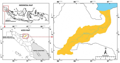
Krueng Pase Watershed is located between 5o09'12 '' - 4o49'25 '' North Latitude and 96o51'27'' - 97o14'55'' East Longitude and the station meteorology is 5o13'4''N; 96o56'5''E. It is located in Lhokseumawe city, Aceh Utara district and Bener Meriah district. (Figure 1). The data used in this study is secondary data obtained from the Meteorology Climatology Geophysics Agency (BMKG), with five variables studied, namely rainfall, total rainy days, humidity, temperature, and duration of irradiation (exposure time). The research variables of rainfall in the Krueng Pase watershed and predictor variables are shown in Table 1.
Table 1. Research variable
|
Symbol |
Variable |
Unit |
Type data |
|
Y |
rainfall |
Millimeter |
Ratio |
|
X1 |
Total Rainy day |
day |
Ratio |
|
X2 |
Temperature |
Celsius |
Interval |
|
X3 |
Humidity |
Percentage |
Ratio |
|
X4 |
Exposure Time |
hour/day |
Ratio |
|
X5 |
Wind velocity |
Knot |
Ratio |
Figure 1. Map of the Krueng Pase watershed area and station Meteorology as the research location
2.2 Analysis
a. Kendall rank correlation analysis
Kendall rank correlation analysis is used to find relationships and test hypotheses between two or more variables if the data is ordinal or ranking value [21]. This method has advantages such as can be used to analyze samples more significant than ten and can be developed to find partial correlation coefficients. The Kendall rank correlation coefficient is given by using the notation $\mid \tau$. The steps taken are (a) ranking the observation data on the $\mathrm{X}$ and $\mathrm{Y}$ variables; (b) Determining $\mathrm{N}$ objects so that $X$ ranks the subjects in good order $1,2,3, \ldots, n$. If there are the same ranking, then the ranking is the average; (c) Observing the Y rank in the order corresponding to the $\mathrm{X}$ rank in the correct order then determine the number of concordant pairs $\left(N_{c}\right)$ and the number of discordant pairs $\left(N_{d}\right)$; (d) Determining the test statistic using the formula (1).
$\tau=2\left(\frac{N_{c}-N_{d}}{N(N-1)}\right)$ (1)
Note:
$\tau=$ Kendall rank correlation coefficient;
$N_{c}=$ number of concordant pairs;
$N_{d}=$ sum of discordant pair numbers;
$N=$ sample size.
$H_{0}$ reject if $\tau>\tau_{\left(N_{c}-N_{d} ; N\right)}$. As for $\mathrm{N}>10$, the distribution used is the normal distribution, by using the formula [18].
$z=\frac{\tau}{\sqrt{\frac{2(2 N+5)}{9 N(N-1)}}}$ (2)
Hereby, $H_{0}$ is rejected if the p-value is less than the significance value. The hypotheses tested are as follows. $H_{0}$ : there is no relationship between the two variables, and $H_{1}$ : there is a relationship between the two variables.
b. Log Transformation in Linear Regression
The virtue of the transformation can minimize skewness and stabilize the value of variance. When the value of the variance changes with the mean based on the strength of the relationship for the positive variable, the Box-Cox class produces the appropriate transformation [22]. The Box-Cox transformation is defined as follows.
$Y^{\prime}=\left\{\begin{array}{l}\ln (Y) \text { for } \lambda=0 \\ \frac{Y^{\lambda}-1}{\lambda} \text { for } \lambda \neq 0\end{array}\right.$ (3)
where is $Y$ the response of the variable in the original scale, $Y^{\prime}$ the response to the variable in the transformation scale, and $\lambda$ is a measure of the strength of the parameter.
Natural log transformations $(\lambda=0)$ are commonly used, the most recent transformation $Y^{\prime}$ will be continued in ANOVA or regression calculations, where the advantage of least squares estimation in efficacy is still hidden $[23,24]$ with the following model:
$\ln (Y)=\beta_{0}+\beta_{1} x_{1}+\ldots+\beta_{k} x_{k}+\varepsilon$. (4)
The response of the transformation $\ln (Y)$ is expressed as a linear function of the predictor variable, $x_{1} x_{k} \varepsilon$ concerning, and the normal distribution and the term homoscedasticity error to estimate the effect of the explanatory variable $(X)$ in the mean of the response variable $Y, E(Y)$, based on multiple linear regression.
$Y=\beta_{0}+\beta X+\beta_{2} X_{2}+\ldots+\beta_{k} X_{k}+\varepsilon, \varepsilon \sim \mathrm{N}\left(0, \sigma^{2}\right)$, (5)
$X_{2}, \ldots, X_{k}$ as other explanatory variables $\beta_{0}$, and $\beta, \beta_{2}, \ldots, \beta_{k}$ unknown parameters are intercepts of the model and regression coefficients $\varepsilon$ are typically distributed residuals. For $Y$ variables without transformation $X$, and $\log$ transformation, the estimate of the median or geometric mean of $Y$ corresponding values $X=x$ is as follows:
$E[Y \mid X=x]=\hat{\beta} \log (x)+\widehat{K}$. (6)
In this calculation, the variable $Y$ is the response, and the variable $X$ is the predictor concerning the effect $X$. It can be said that the measure is independent of both values $X \widehat{K}$. The additive change in cunits $X$ is the result of a relative change in the median or geometric mean of $Y$ or equivalent [25].
$\Delta \widehat{M} \%=100 \frac{\widehat{M}[Y \mid X=x+c]-\widehat{M}[Y \mid X=x]}{\widehat{M}[Y \mid X=x]}$$=100\left(e^{\widehat{\beta} c}-1\right) \%$, (7)
c. Normality, multicollinearity, heteroscedasticity, and autocorrelation tests
The normality test aims to test whether the confounding or residual variables have a normal distribution in the regression model to detect whether the residuals are normally distributed or not, the one-sample Kolmogorov-Smirnov test is carried out with a decision-making basis, namely [26, 27]: (a) If the results of the one-sample Kolmogorov-Smirnov are above the 0.05 level of significance, it shows the distribution pattern. Then the regression model meets the normality assumption; (b) If the Kolmogorov-Smirnov one-sample result below the 0.05 level of significance does not indicate a typical distribution pattern, then the regression model does not meet the assumption of normality.
The next step is to do a multicollinearity test to determine whether there is a correlation between the independent variables in the regression model. Detection of the presence or absence of multicollinearity in the regression model can be seen from the tolerance value and variance inflation factor (VIF).
A heteroscedasticity test was carried out to test whether there was an inequality of variance from the residuals of one observation to another observation in the regression model. If the variance from the residual of one observation to another remains, it is called homoscedasticity, and if it is different, it is called heteroscedasticity [28]. An autocorrelation test was carried out to test whether in the linear regression model there was a correlation between the confounding error in the period tt-1 and is the error in the (previous) period.
$F=\frac{\frac{\sum_{i=1}^{K} n_{i}\left(\bar{Y}_{i .}-\bar{Y}\right)^{2}}{(K-1)}}{\frac{\sum_{i=1}^{K} \sum_{j=1}^{n_{i}}\left(Y_{i j}-\bar{Y}_{i .}\right)^{2}}{(N-K)}}$ (8)
This test produces calculated DW (d) and Durbin Watson table values (dl and du). Decision-making related to the presence or absence of autocorrelation through the DW table criteria with a significance level of 5% and four independent variables (k=4) [9]. It is an overall regression model test that determines whether the model made is feasible to be a good model. The test is carried out by calculating ANOVA to obtain the F value as follows [29-31].
Root Mean Square Error (RMSE) is used to calculate the error rate of the two experimental models. The amount of RMSE value can be calculated by the following equation [32].
$R M S E=\sqrt{M S E}=\sqrt{\frac{1}{M} \sum_{l=1}^{M}\left(Z_{n+l}-\hat{Z}_{n}(l)\right)^{2}}$ (9)
The $M$ is the number of predictions made, while $Z_{n+1}$ is the actual data and $\hat{Z}_{n}(l)$ the forecast data.
In the first step of the research, data exploration was carried out using descriptive statistics and graphic visualization. Data exploration is needed to determine the characteristics of the data [28, 29] so that it can determine or apply the appropriate analysis method. The characteristics of the rainfall data and the influencing factors consisting of Rainy Days, Temperature, Humidity, Wind Speed, and Length of Radiation in the Krueng Pase Watershed in North Aceh Regency from January to December between 1992 and 2020 (Table 2).
Based on Table 2, it can be seen that the characteristics of the data studied had been explained by using the average value (mean), the distribution of the data contained in the sample (standard deviation), the minimum value (min), the maximum value (max), the slope of the distribution (skewness) and the sharpness of the distribution (kurtosis). The value of skewness and kurtosis indicates the degree of asymmetry of a distribution. Table 2 indicates that the rainfall variable has the most significant standard deviation value of 89.45 mm, followed by the wind speed variable of 54.55 knots. This shows that the two variables have the most considerable variance among other variables with relatively small standard deviation.
Table 2. Descriptive statistics of rainfall changes
|
Variable |
Mean |
Deviation Standard |
Min |
Max |
Skewness |
Kurtosis |
|
Rainfall (1) |
118.3 |
89.45 |
2 |
571 |
1.53 |
3.16 |
|
Rainy day (2) |
14.557 |
5.691 |
2 |
29 |
0.15 |
-0.55 |
|
Temperature (3) |
26.782 |
1.125 |
24.9 |
34.819 |
2.66 |
13.28 |
|
Humidity (4) |
81.338 |
3.876 |
70.733 |
94 |
-0.18 |
-0.14 |
|
Exposure time (5) |
6.2704 |
1.2514 |
0.7 |
9.2 |
-0.57 |
0.93 |
|
Wind Velocity (6) |
125.27 |
54.55 |
10 |
360 |
1.48 |
5.28 |
Based on Table 2, it also shows that the humidity and irradiation time (exposure time) variables have a skewness value of -0.18 and -0.57, respectively, where the value is below 0, which indicates that the data has a slope to the right and shows that the distribution of the data is not symmetrical and has negative skewness. While the variables of rainfall, rainy days, temperature, and wind speed showed a skewness value greater than 0, indicating that the data had a slope to the left and indicated that the data distribution was not symmetrical and had a positive skewness. Lastly, the kurtosis value on a rainy day and humidity variables with (k) < 0 is -0.55, and -0.14 indicates that the data is much heterogeneous. This also implies that the other variables have homogeneous data. The visualization of the skewness and kurtosis shows by Figure 2, indicates that all the variables are not normally distributed.
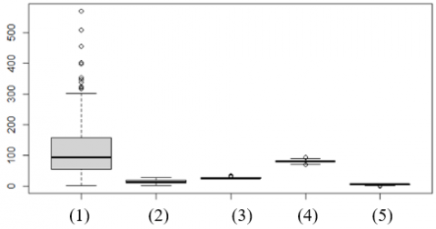
Based on Figure 3, it is found that there are outliers in the variables of rainfall, temperature, humidity, and duration of irradiation, so it is necessary to pre-process the data to minimize bias analysis. The boxplot in Figure 3 also indicates that the rainfall variable has an enormous variance value compared to other variables. Boxplot visualization also shows the value of Quartile 1, Median (middle value), Quartile 3, minimum value (smallest observation value), and maximum value (most considerable observation value). In this study, it can be seen that all the variables studied have different characteristics.
Based on Figure 4, it is known that all the variables studied are not normally distributed. This is indicated by P-Value < 0.05, where H0 had been rejected, which means the data is not normally distributed. A transformation log can help the distribution become more normalized [31]. Through visualization, it can also be seen that the distribution of plotting points is not on a diagonal line, so it is necessary to transform the data to meet the assumption of normality [32, 33]. Abnormalities in the data are due to outlier values or extreme values in a data set, resulting in a skewness distribution (skew) in the analyzed data.
The data used in this study is continuous in the period 1992 to 2020, so that the abnormal distribution can also be caused by differences in the shape of the distribution. There is overlap in the data so that round-off errors or measurement devices with low resolution can make it true. It is true that continuous data and normally distributed data look discrete and not expected.
Correlation Analysis with Kendall-Tau aims to measure the strength of the relationship between the variables studied as well as to determine whether there is a relationship among variables [21]. In this study, correlation analysis was used to determine the relationship between rainfall and the influencing factors in the Krueng Pase Watershed in North Aceh Regency. The analytical method used in this study is the Kendall-Tau correlation with the following output (Table 3).
Based on Table 3, it can be seen that all variables have P-Value < 0.01, indicating that there is a relationship among all predictor variable (rainy day, temperature, humidity, and Exposure time /duration of irradiation) to the response variable (rainfall). The exception is for the wind speed that has no relationship to other variables, so that the wind speed variable is not used in subsequent regression analysis. The strength of the correlation can also be known through the value of the correlation coefficient, if the value is close to 1, it is indicated to have a very strong correlation.
The results of the analysis of data characteristics found that all variables were not normally distributed, so it was necessary to transform them to make assumptions [34, 35]. The analytical method used is Log Transformation Linear Regression, and the output can be seen in (Table 4).
The statistical theory used to develop the classic techniques for constructing confidence intervals for population means and performing statistical tests of hypotheses begins with the assumption that the response of interest has a normal distribution. If this assumption is true, inferences from the results are valid (e.g., statistical significance of P values and width of confidence intervals). One common type is the logarithmic transformation. If the data are continuous and nonnegative and have a positively skewed distribution, they may have a distribution that is referred to as log normal [26].
Figure 2. Distribution plot for all variables
Figure 3. Boxplot visualization on all variables
Figure 4. Visualization of probability plots on all variables studied
Simple Linear Regression shows the pattern of relationship between X and Y variables. The X variable consisted of rainy days, temperature, humidity, and exposure time. Variable Y is rainfall. Linear regression is used to predict quantitative outcomes based on a single variable on a single predictor by constructing a mathematical model defined as a function of the variables. The prediction results using simple linear regression can be seen in Table 4. The Coefficients column can be seen as follows:
$Y=826.92+82.27 X_{1}-116.94 X_{2}-135.59 X_{3}+21.22 X_{4}$
The model represents; Y= rainy day as the variable response. And other variables are X1 = rainy day, X2 = temperature, X3= humidity, and X4 = Exposure time. The regression equation above explained that, if other variables are constant, the value of rainfall will change automatically by a constant value of 826.92. If other variables are constant, the value of Rainy Days will change by 82.27 per unit, Temperature by -116.94, Humidity by -135.59, and the irradiation time of 21.22 per unit. The increase of 1 rainy day will increase the rainfall about 82.27mm, the increase of 1℃ temperature will decrease the Y by 116.94 mm.
Table 5 shows the results of the F test. It’s used to predict the contribution of the independent variable (X) to the dependent variable (Y). Using a confident interval of 95% and an error value of 5%, the P-Value <0.05, which means rejecting H0, indicates that the regression model is linear. It shows that the regression model Y to X is significant.
The regression results in Table 4 indicated that the variables of rainy days, temperature, humidity, and Exposure time have a relationship with rainfall.
Linear regression analysis must meet several assumptions, including normality, multicollinearity, heteroscedasticity, and autocorrelation. Normality test aims to assess the distribution of data in a group of variables. In multiple linear regression analysis, the normality test was carried out for the residual results that have been analyzed.
The homoscedasticity tests the similarity of variance from the residual observations to others in the regression model. It means that heteroscedasticity is the opposite of homoscedasticity. A good regression model is one with homoscedasticity without any heteroscedasticity. The following is the output of the normality test using the Kolmogorov Smirnoff with an alpha value of 0.05 and a homoscedasticity test.
The generalized linear model (GLM) equation cannot be interpreted as a normal regression [24, 35] because the model has an exponential. It requires a "DHARMA" approach that simulates GLM as an ordinary linear regression equation [36]. Based on Figure 5 on the QQ plot of residuals, it can be seen that the residuals through regression testing meet the normal distribution. From the graph, it can also be seen that the Kolmogorov Smirnov test obtained P-Value > 0.05 indicates that the residuals are normally distributed.
Table 3. Correlation analysis with Kendall-tau
|
|
Rainfall |
Rainy day |
Temperature |
Humidity |
Exposure time |
Wind velocity |
|
|
Rainfall |
Correlation Coefficient |
1.000 |
.401** |
-.204** |
.323** |
-.235** |
-.023 |
|
Sig. (2-tailed) |
. |
.000 |
.000 |
.000 |
.000 |
.562 |
|
|
N |
348 |
348 |
348 |
348 |
348 |
348 |
|
|
Rainy day |
Correlation Coefficient |
.401** |
1.000 |
-.262** |
.329** |
-.322** |
.032 |
|
Sig. (2-tailed) |
.000 |
. |
.000 |
.000 |
.000 |
.427 |
|
|
N |
348 |
348 |
348 |
348 |
348 |
348 |
|
|
Temperature |
Correlation Coefficient |
-.204** |
-.262** |
1.000 |
-.365** |
.191** |
-.052 |
|
Sig. (2-tailed) |
.000 |
.000 |
. |
.000 |
.000 |
.181 |
|
|
N |
348 |
348 |
348 |
348 |
348 |
348 |
|
|
Humidity |
Correlation Coefficient |
.323** |
.329** |
-.365** |
1.000 |
-.218** |
-.194** |
|
Sig. (2-tailed) |
.000 |
.000 |
.000 |
. |
.000 |
.000 |
|
|
N |
348 |
348 |
348 |
348 |
348 |
348 |
|
|
Exposure time |
Correlation Coefficient |
-.235** |
-.322** |
.191** |
-.218** |
1.000 |
-.077* |
|
Sig. (2-tailed) |
.000 |
.000 |
.000 |
.000 |
. |
.050 |
|
|
N |
348 |
348 |
348 |
348 |
348 |
348 |
|
|
Wind velocity |
Correlation Coefficient |
-.023 |
.032 |
-.052 |
-.194** |
-.077* |
1.000 |
|
Sig. (2-tailed) |
.562 |
.427 |
.181 |
.000 |
.050 |
. |
|
|
N |
348 |
348 |
348 |
348 |
348 |
348 |
|
**. Correlation is significant at the 0.01 level (2-tailed).
*. Correlation is significant at the 0.05 level (2-tailed).
Table 4. Coefficient of log transformation linear regression
|
Estimate |
Std. Error |
t-value |
Pr(>|t|) |
|
|
(Intercept) |
826.92 |
591.93 |
1.397 |
0.1635 |
|
Rainy day |
82.27 |
8.81 |
9.338 |
< 0.01 *** |
|
Temperature |
-116.94 |
133.52 |
-0.876 |
0.3819 |
|
Humidity |
-135.59 |
78.23 |
-1.733 |
0.0842 |
|
Exposure Time |
21.22 |
21.38 |
0.993 |
0.3217 |
Table 5. Residual and ANOVA
|
Min |
1st Q |
Median |
3rd Q |
Max |
R2 |
Adj (R2) |
F |
P |
|
-123.052 |
-38.397 |
-9.139 |
32.077 |
200.669 |
0.2461 |
0.2352 |
22.53 |
< 0.05 |
Based on Figure 5 on the prediction plot model, it is known that the data distribution pattern spreads evenly and homoscedasticity pattern, which means it does not form a certain pattern. Through this analysis, it can be seen that the model meets the assumptions of normality and homoscedasticity. The next test is multi-collinearity with the value of Variance Inflation Factor (VIF) (X1) 1.032099; (X2) 1.022586; (X3) 1.049068; (X4) 1.013003. The model simulation using generalized linear bivariate produces good performance for future and past rainfall [37]. Prediction of rainfall is highly dependent on physical phenomena and atmospheric conditions as well as mathematical models.
Figure 5. DHARMA residual diagnostics
Multicollinearity (Double Collinearity) is the existence of a perfect or definite linear relationship between or several independent variables (explanatory) from multiple linear regressions. The multicollinearity test aims to identify the occurrence of multicollinearity in multiple linear regression analysis. The value of the Variance Inflation Factor in each predictor variable. The multicollinearity test found that all predictor variables had a VIF value below 10, indicating that there was no multicollinearity in the data. It can be concluded that the model meets the multicollinearity assumption in the data. The next test is autocorrelation using Durbin Watson with DW (2.0104) and P-value (0.4871).
Autocorrelation in the concept of linear regression means that the error component correlated with the time sequence (periodic data or within a certain period). In other words, autocorrelation is a correlation in itself. The classical linear regression method assumes that autocorrelation does not occur. Through testing with the Durbin-Watson test, the p-value > 0.05 indicates no influence between the previous and latest data, so it can be concluded that the model meets the correlation assumption.
Rainfall prediction using log transformation obtained R2 of 24.61%. The Box-Jenkins approach is applied to the SARIMA model. Experimental results show that rainfall will not change in the future unless there are some human and industrial activities that interfere with it [17]. Rainfall predictions from past events that are too long produce poor predictions [14].
In general, the log transformation can reduce the variability of the data and make the data more fit close to the normal distribution. However, the log-transformed data is often irrelevant for the original untransformed data [38]. Since climate change has begun to occur in the Krueng Peusangan, there might be more other factors influence it to be related to climate data. The model made by this method depends on the data (in case Krueng Pase watershed) obtained, and the possibility of irrelevance might be increased. However, using more relevant variables and updated dataset shall reduce this kind of weakness, and this method will be a great tool. Alternatively, a spatio-temporal model is needed to estimate the complex climatological distribution using the normal distribution [39]. To strengthen the results of the analysis conducted model accuracy testing using RMSE and obtained for the Log-Transformation linear regression model method with an RMSE value of 57.67584.
Weather forecasting is an application of knowledge and technology that is used to predict rainfall in the future depending on input attributes. Historical data used in several studies to predict rainfall are temperature, wind speed, wind direction, humidity and atmospheric pressure [40]. In this study, we consider rainy days to predict rainfall forecasting is a scientifically and technologically challenging problem. Many forecasters are in the health sector, trade and meteorology. For forecasting can be done through an empirical approach and a dynamic approach. Empirical approach based on historical analysis of rainfall and the relationship with various atmospheric variables using regression methods, artificial neural networks, fuzzy logic and data collection groups. The dynamic approach is implemented using the numerical rainfall forecasting method on a large scale and long term [41].
The rainfall-runoff process is an essential part of the hydrological cycle and explains the transformation of rainfall into river discharge. River discharge in the catchment is influenced by many interrelated processes. Heterogeneity is one of the transformation processes such as heterogeneity of the transformation process of temperature and humidity variables into rainfall. Rainfall prediction becomes a consideration in discharge calculation.
Climate also affects the evapotranspiration from hydrology cycle. One of the studies that explore the performance of rainfall and Evapotranspiration (ETo) data from the global European Centre for Medium-Range Weather Forecasts found that the comparison between ETo and flow time series exhibit a similar variability for the whole hydrologic year and follow a strong seasonal cycle. The peak normal evapotranspiration occurred from January to February because of a very high wet soil profile and low ETo during the period of December to February Similar interpretation can be observed from ETo and flow time series, like temperature increased and high evaporation through the period April–May to August–September led to a progressive soil drying [6].
In many cases especially in areas where accurate data collection is difficult, reliable ETo estimates derived from Thornthwaite method can be used to calculate the ETo when temperature is the only input parameter available. In such cases, it will be a good consideration to compare and validate with other methods based on the precise evaluation considering the land coverage and topographical condition to reduce the range of uncertainty [42]. Rainfall–baseflow and runoff models based on flow logarithms provide a good representation of the baseflow for the catchment based on rainfall prediction [43, 44]. So that the initial step for the prediction of rainfall as a climate variable is very much needed for the accuracy of the prediction of discharge and its relation to land use changes.
Linear regression test by using log transformation obtained R2 of 24.61% with an RMSE value of 57,676. The rainfall regression equation (Y) will change by itself at a constant value of 826.92 and if other variables are constant then the value of Rainy Days will change by 82.27 per unit, The temperature is -116.94, the humidity is -135.59, and the irradiation time is 21.22 per unit. It indicates an influence between rainfall and other influencing factors such as rainy days, temperature, humidity, and duration of irradiation. Wind speed at the research location has no relationship with other variables because it has a no significant correlation value. The overall analysis was found that the model meets the classical assumptions. Other variables also need to be considered in the subsequent analysis, such as regional characteristics that affect climate (geographical location, altitude, and eco-hydrology related land use conditions. It will also strengthen the results of the study. In the research method, it is necessary to compare all the available methods to find the best method in modeling the relationship between rainfall and the factors that influence it. The method suggested in the following research is a nonlinear method.
We thank to BMKG Indrapuri Aceh for the data provided and Universitas Syiah Kuala for funding this research, Contract No. 167/UN11/SPK/PNBP/2021, 19 February 2021.
[1] Islam, T., Rico-Ramirez, M.A., Han, D., Srivastava, P.K. (2012). A Joss–Waldvogel disdrometer derived rainfall estimation study by collocated tipping bucket and rapid response rain gauges. Atmospheric Science Letters, 13(2): 139-150. https://doi.org/10.1002/asl.376
[2] Handayani, W., Chigbu, U.E., Rudiarto, I., Putri, I.H.S. (2020). Urbanization and increasing flood risk in the northern coast of central java—Indonesia: An assessment towards better land use policy and flood management. Land, 9(10): 343. https://doi.org/10.3390/land9100343
[3] Caldas, A.M., Pissarra, T.C.T., Costa, R.C.A., Neto, F.C.R., Zanata, M., Parahyba, R.D.B.V., Fernandes, L.F.S., Pacheco, F.A.L. (2018). Flood vulnerability, environmental land use conflicts, and conservation of soil and water: A study in the Batatais SP municipality, Brazil. Water, 10(10): 1357. https://doi.org/10.3390/w10101357
[4] Srivastava, P.K., Han, D., Rico-Ramirez, M.A., Islam, T. (2014). Sensitivity and uncertainty analysis of mesoscale model downscaled hydro‐meteorological variables for discharge prediction. Hydrological Processes, 28(15): 4419-4432. https://doi.org/10.1002/hyp.9946
[5] Amatya, D.M., Sun, G., Skaggs, R.W., Chescheir, G.M., Nettles, J.E. (2006). Hydrologic effects of global climate change on a large drained pine forest. In Hydrology and Management of Forested Wetlands, Proceedings of the International Conference, April 8-12, New Bern, North Carolina, p. 46.
[6] Srivastava, P.K., Han, D., Rico-Ramirez, M.A., Islam, T. (2014). Sensitivity and uncertainty analysis of mesoscale model downscaled hydro‐meteorological variables for discharge prediction. Hydrological Processes, 28(15): 4419-4432. https://doi.org/10.1002/hyp. 9946
[7] Abdullah, S., Ismail, M. (2019). The weather and climate of tropical Tasik Kenyir, Terengganu. In Greater Kenyir Landscapes, pp. 3-8. https://doi.org/10.1007/978-3-319-92264-5
[8] Ramli, I., Rusdiana, S., Basri, H., Munawar, A.A. (2019). Predicted rainfall and discharge using vector autoregressive models in water resources management in the high hill Takengon. In IOP Conference Series: Earth and Environmental Science, 273(1): 012009. https://doi.org/10.1088/1755-1315/273/1/012009
[9] Chang, T.K., Talei, A., Alaghmand, S., Ooi, M.P.L. (2017). Choice of rainfall inputs for event-based rainfall-runoff modeling in a catchment with multiple rainfall stations using data-driven techniques. Journal of Hydrology, 545: 100-108. https://doi.org/10.1016/j.jhydrol.2016.12.024
[10] Vose, J.M., Sun, G., Ford, C.R., Bredemeier, M., Otsuki, K., Wei, X.H., Zhang, Z.Q., Zhang, L. (2011). Forest ecohydrological research in the 21st century: what are the critical needs? Ecohydrology, 4(2): 146-158. https://doi.org/10.1002/eco.193
[11] Zalewski, M. (2006). Flood pulses and river ecosystem robustness. IAHS Publications-Series of Proceedings and Reports, 305: 143-154.
[12] Achmad, A., Irwansyah, M., Nizamuddin, N., Ramli, I. (2019). Land use and cover changes and their implications on local Climate in Sabang City, Weh Island, Indonesia. Journal of Urban Planning and Development, 145(4): 04019017. https://doi.org/10.1061/(ASCE)UP.1943-5444.0000536
[13] Ichwana, Chairani, S., Ahmad, A. (2015). Climate trends and dynamic change of land use patterns in Krueng Peusangan watershed. Aceh-Indonesia Change, symposium on Geoinformatis, International Symposium on geoinformatics, Faculty of Computer Science (FILKOM F.ka PTIIK) Universitas Brawijaya.
[14] Ramli, I., Rusdiana, S., Achmad, A. (2019). Comparisons among rainfall prediction of monthly rainfall basis data in Aceh using an autoregressive moving average. In IOP Conference Series: Earth and Environmental Science, 365(1): 012008. https://doi.org/10.1088/1755-1315/365/1/012008
[15] Shortridge, J.E., Guikema, S.D., Zaitchik, B.F. (2016). Machine learning methods for empirical streamflow simulation: A comparison of model accuracy, interpretability, and uncertainty in seasonal watersheds. Hydrology and Earth System Sciences, 20(7): 2611-2628. https://doi.org/10.5194/hess-20-2611-2016
[16] Zhang, W., Zhang, H., Liu, J., Li, K., Yang, D., Tian, H. (2017). Weather prediction with multiclass support vector machines in the fault detection of photovoltaic system. IEEE/CAA Journal of Automatica Sinica, 4(3): 520-525. https://doi.org/10.1109/JAS.2017.7510562
[17] Singhrattna, N., Rajagopalan, B., Clark, M., Krishna Kumar, K. (2005). Seasonal forecasting of Thailand summer monsoon rainfall. International Journal of Climatology: A Journal of the Royal Meteorological Society, 25(5): 649-664. https://doi.org/10.1002/joc.1144
[18] Dutta, P.S., Tahbilder, H. (2014). Prediction of rainfall using data mining technique over Assam. Indian Journal of Computer Science and Engineering (IJCSE), 5(2): 85-90.
[19] Maran, P.S., Ponnusamy, R. (2013). Short term estimation and analysis of wind speed using data mining techniques. International Journal of Computer Applications (0975 – 8887) International Conference on Computing and information Technology.
[20] Pek, J., Wong, O., Wong, A.C. (2017). Data transformations for inference with linear regression: Clarifications and recommendations. Practical Assessment, Research, and Evaluation, 22(1): 9. https://doi.org/10.7275/2w3n-0f07
[21] Newson, R. (2002). Parameters behind “non-parametric” statistics: Kendall’s tau, Somers’ D and median differences. Stata Journal, 2(1): 45-64.
[22] Conover, W.J. (1971). Pratical Nonparametric Statistic. New York: Jhon Wiley & Son, 256.
[23] Box, G.E., Cox, D.R. (1964). An analysis of transformations. Journal of the Royal Statistical Society: Series B (Methodological), 26(2): 211-243. https://doi.org/10.1111/j.2517-6161.1964.tb00553.x
[24] Gomez, J.B., Basagana, X. (2014). Supplemental Material for “Models with transformed variables: interpretation and software”. Epidemiology, pp. 5-9. https://doi.org/10.1097/EDE.0000000000000247
[25] Fox, J. (2015). Applied Regression Analysis and Generalized Linear Models. Sage Publications.
[26] Olivier, J., Johnson, W.D., Marshall, G.D. (2008). The logarithmic transformation and the geometric mean in reporting experimental IgE results: What are they and when and why to use them? Annals of Allergy, Asthma & Immunology, 100(4): 333-337. https://doi.org/10.1016/S1081-1206(10)60595-9
[27] Steinskog, D.J., Tjøstheim, D.B., Kvamstø, N.G. (2007). A cautionary note on the use of the Kolmogorov–Smirnov test for normality. Monthly Weather Review, 135(3): 1151-1157. https://doi.org/10.1175/MWR3326.1
[28] Lomax, R.G. (2007). An introduction to statistical concepts. Lawrence Erlbaum Associates Publishers.
[29] Box, G.E.P., Jenkins, G. M., Reinse, G.C. (1994). Time Series Analysis: Forecasting and Control, 3rd ed. Prentice-Hall, Old Tappan.
[30] Bowerman, B.L., O'Connell, R.T., Koehler, A.B. (2005). Forecasting, time series, and regression. United States of America: Curt Hinrichs.
[31] Bland, J.M., Altman, D.G. (1996). Statistics notes: the use of transformation when comparing two means. Bmj, 312(7039): 1153. https://doi.org/10.1136/bmj.312.7039.1153
[32] William, W.S. (2006). Time Series Analysis Univariate and Multivariate Methods. New York: Pearson Education Inc.
[33] Lima, A.R., Cannon, A.J., Hsieh, W.W. (2015). Nonlinear regression in environmental sciences using extreme learning machines: A comparative evaluation. Environmental Modelling & Software, 73: 175-188. https://doi.org/10.1016/j.envsoft.2015.08.002
[34] Feng, C.Y., Wang, H.Y., Lu, N.J., Chen, T., He, H., Lu, Y., Tu, X.M. (2014). Biostatistics in Psychiatry Shanghai Archives of Psychiatry.
[35] Curran-Everett, D. (2018). Explorations in statistics: the log transformation. Advances in Physiology Education, 42(2): 343-347. https://doi.org/10.1152/advan.00018.2018
[36] Gad, A.M., El Kholy, R.B. (2012). Generalized linear mixed models for longitudinal data. International Journal of Probability and Statistics, 1(3): 41-47. https://doi.org/10.5923/j.ijps.20120103.03
[37] George, J., Letha, J., Jairaj, P.G. (2016). Daily rainfall prediction using generalized linear bivariate model–a case study. Procedia Technology, 24: 31-38. https://doi.org/10.1016/j.protcy.2016.05.006
[38] Hartig, F. (2020). DHARMa: residual diagnostics for hierarchical (multi-level/mixed) regression models. R package version 0.3, 3.
[39] Stauffer, R., Mayr, G.J., Messner, J.W., Umlauf, N., Zeileis, A. (2017). Spatio-temporal precipitation climatology over complex terrain using a censored additive regression model. International Journal of Climatology, 37(7): 3264-3275. https://doi.org/10.1002/joc.4913
[40] Anusha, N., Chaithanya, M.S., Reddy, G.J. (2019). Weather prediction using multi linear regression algorithm. In IOP Conference Series: Materials Science and Engineering, 590(1): 012034. https://doi.org/10.1088/1757-899X/590/1/012034
[41] Latha, C.B.C., Paul, S., Kirubakaran, E., Sathianarayanan, A. (2010). A service oriented architecture for weather forecasting using data mining. Int. J. of Advanced Networking and Applications, 2(2): 608-613.
[42] Ma, J. (2006). Comparison of several reference evapotranspiration methods for Itoshima Peninsula area, Fukuoka, Japan. Memoirs of the Faculty of Engineering, Kyushu University, 66(1): 1-15.
[43] Pek, J., Wong, A.C.M., Wong, O.C.Y. (2017). Construction of accurate confidence intervals for the mean of non-normally distributed data. Open Journal of Statistics, 7(3): 405-421. https://doi.org/10.4236/ojs.2017.73029
[44] Nasution, Z., Ichwana, Sumono, Delvian. (2013). Land-use change and simulation of hydrological response using integrated NRCS model and base flow for the ecohydrological concept at Krueng Peusangan watershed, Aceh, Indonesia. Journal of Environmental Science and Water Resources, 2(7): 210-220. https://www.wudpeckerresearchjournals.org/JESWR/pdf/2013/August/Nasution%20et%20al.pdf.