Gabriel Onuche Odekina* | Adedayo Funmi Adedotun | Oluwaseun Ayodeji Odusanya
© 2021 IIETA. This article is published by IIETA and is licensed under the CC BY 4.0 license (http://creativecommons.org/licenses/by/4.0/).
OPEN ACCESS
With the outbreak of COVID-19, a lot of studies have been carried out in various science disciplines to either reduce the spread or control the increasing trend of the disease. Modeling the outbreak of a pandemic is pertinent for inference making and implementation of policies. In this study, we adopted the Vector autoregressive model which takes into account the dependence that exists between both multivariate variables in modeling and forecasting the number of confirmed COVID-19 cases and deaths in Nigeria. A co-integration test was carried out prior to the application of the Vector Autoregressive model. An autocorrelation test and a test for heteroscedasticity were further carried out where it was observed that there exists no autocorrelation at lag 3 and 4 and there exists no heteroscedasticity respectively. It was observed from the study that there is a growing trend in the number of COVID-19 cases and deaths. A Vector Autoregressive model of lag 4 was adopted to make a forecast of the number of cases and death. The forecast also reveals a rising trend in the number of infections and deaths. The government therefore needs to put further measures in place to curtail the spread of the virus and aim towards flattening the curve.
COVID-19, co-integration, vector autoregressive model
The corona virus disease known as a form of severe acute respiratory syndrome was initially discovered in the city of Wuhan, China in 2019, December precisely and it was acknowledged as a pandemic by World Health Organization [1] on the 11th of March 2020 after infecting over 118,000 people globally. The virus which has spread at an exponential rate all over the world has negatively affected the healthcare system in many countries. The COVID-19 pandemic is one of the worst pandemics mankind has ever been confronted after the Spanish flu pandemic in 1918, which caused the deaths of about 50 million people at a time the world’s population was around 2 billion.
In Nigeria, the first known and confirmed case of COVID-19 was documented on the 27th of February 2020 in Lagos state according to Nigeria Center for Disease Control [2]. After the index case on the 27th of February, the number of confirmed cases has been on the rise with the earliest reported death case on 22nd March 2020. Due to the speedy escalation in the number of cases in Nigeria, the Federal government had to enforce total lockdown in Lagos, Abuja and Ogun state. Some states which were not included in the total lockdown by the federal government also had lockdown enforced by the state Government in order to curtail the rise of the deadly virus. With the outbreak of COVID-19, a lot of studies have been carried out in various science disciplines to either reduce the spread or control the increasing trend of the disease. Therefore, in order to manage and comprehend the epidemic, various approaches of estimation, modelling and forecasting have been introduced.
Zeroual et al. [3] carried out a relative study to project the new number of COVID-19 reported cases and recovered cases based on 5 deep learning methods. Precisely, Long Short-Term Memory (L STM), Gated recurrent units (GRUs), simple Recurrent Neural Network (RNN), Variational Auto-Encoder (VAE) algorithms and Bidirectional L STM (BiL STM) were used for the global foretelling of COVID-19 cases with respect to a petty amount of data. Their study is based on daily verified cases and the number of cases recovered obtained from six different countries which are China, Spain, Italy, Australia, USA, and France. The performance of each model was verified where it was observed that VAE has a better forecasting precision when compared to the other models used.
Forecasting the Coronavirus (COVID-19) cases and deaths, Petropoulos et al. [4] proposed the approach of statistical time series to model and forecast the short period behavior of COVID-19. Petropoulos et al. [4] assumed a trend that is multiplicative which aims to capture the persistence of the two variables predicted (number of cases and mortality rate) as well as their uncertainty. The anticipated time series model showed an excellent level of precision and ambiguity as additional data were collected.
Ribeiro et al. [5] evaluated random forest (RF), ridge regression (RIDGE), autoregressive integrated moving average (ARIMA), stacking-ensemble learning, support vector regression (SVR) and cu-bist regression (CUBIST) in the charge of time series forecasting with one, three, and six-days ahead the COVID-19 increasing established cases in ten Brazilian states with a soaring daily incidence. Within the stacking-ensemble learning approach, the RIDGE, CUBIST regression, SVR and RF models were adopted as base-learners and Gaussian process (GP) as meta-learner. The efficiency of the models was evaluated base on the mean absolute error, absolute percentage error criteria, symmetric mean, and improvement index. In majority of the cases, the stacking-ensemble learning and SVR achieve an improved performance as regards the adopted criteria than compared models. Generally, the developed models can make precise forecasting, achieve errors in a range of 0.87%–3.51%, 1.02%–5.63% and 0.95%–6.90% in one, three, and six-days-ahead respectively. In the study of statistical analysis of COVID-19 using the Gaussian and probabilistic model by Nayak et al. [6], it was observed that all countries have a higher recovery rate than death rate apart from UK where the death rate is greater than the rate of recovery. The Gaussian model applied was able to forecast the maximum numbers of the confirmed cases.
de Figueiredo et al. [7] studied the effect of total lockdown on COVID-19 prevalence rate and death rate in China where it was advised that lockdown is effective in reducing the incidence rate and mortality rate. Maleki et al. [8] modeled and forecasted the increase of COVID-19 and death that has occurred as a result of corona-virus disease in the world. The distributions of the error were well thought-out to be two-member scale mixture of traditional (TP-SMN) where the model that has the most excellent fit was carefully chosen. The chosen model was used to forecast the number of cases and death of COVID-19 in the world at large. Maleki et al. [8] also examined a time series model which was used to project the verified number of cases and recuperated cases of the corona virus disease.
Dehkordi et al. [9] examined the epidemic data and Statistics with focus on COVID-19 where it was observed in the study that some policies which prove effective were the lockdown measures in Italy, Spain and China and the shutdown of companies in Hubei offering non-essential services.
In the study carried out on the coronavirus (COVID-19) in Spain and Italy by Chu [10], two simple mathematical epidemiological models were applied where it was observed that the log-linear regression yielded an improved result and basic estimate of the everyday incidence for both countries.
Olusola-Makinde and Makinde [11] studied the gender based COVID-19 prevalence rate and death rate in Nigeria. In the study, a Wilcoxon signed-rank test was adopted to examine disparity in the sex distributions of the daily prevalence. A VARMA model of a variety of orders was framed for the gender based daily COVID-19 incidence in Nigeria. The best VARMA model was recognized by means of Bayesian information criterion. In addition, a predictive model based on a univariate autoregressive moving average model was developed for the daily death cases in Nigeria. In the work [12], the autoregressive integrated moving average was adopted to forecast the COVID-19 incidence rate in India where an increasing tendency in the number of corona virus cases was observed.
Modeling the outbreak of a pandemic is pertinent for inference making and implementation of policies. In this paper, we adopted the Vector autoregressive model in modeling and forecasting the number of COVID-19 cases and deaths in Nigeria. A co-integration test was carried out prior to the application of the Vector Autoregressive model.
2.1 Data source
The data used for this study is a daily data on the number of COVID-19 cases and death obtained from https://raw.githubusercontent.com/owid/covid-19-data/master/public/data/owid-covid-data.xlsx.
The methodology used for this paper is given below.
2.2 Co-integration model
This model deals with two or more non-stationary variables whose linear combination of the variables gives an integration of order zero I (0). That is, the linear combination of the non-stationary variables results into stationary. It creates a link among two or more non-stationary series by finding a linear combination which gives an integration of order zero.
Consider a k-dimensional vector autoregressive model of order 2 given below, where $a_{t} \sim N(0, \Sigma)$, $\Phi_{1}$ and $\Phi_{2}$ are $\mathrm{k} \times \mathrm{k}$ matrices of unknown coefficients.
${{y}_{t}}={{\Phi }_{1}}{{y}_{t-1}}+{{\Phi }_{2}}{{y}_{t-2}}+{{a}_{t}}$ (1)
Subtracting yt-1 from both sides of Eq. (1), and adding Φ2yt-1 to the right hand side of Eq. (1), we have:
$\Delta y_{t}=\Phi y_{t-1}+\Gamma \Delta y_{t-1}+a_{t}, \mathrm{t}=1,2, . . \mathrm{T}$ (2)
where,
Eq. (2) is referred to as the vector error correction model, otherwise called the co-integrated vector autoregressive model. Suppose we have a multivariate variable consisting of variables P and Q, according to Juselius [13], Eq. (2) can be written in matrix form as:
$\left[ \begin{matrix} \Delta P \\ \Delta Q \\\end{matrix} \right]=\left[ \begin{matrix} {{P}_{11}} & {{P}_{12}} \\ {{P}_{21}} & {{P}_{22}} \\\end{matrix} \right]\left[ \begin{matrix} \Delta {{P}_{t-1}} \\ \Delta {{Q}_{t-1}} \\\end{matrix} \right]+\left[ \begin{matrix} {{\beta }_{11}} & {{\beta }_{12}} \\ {{\beta }_{21}} & {{\beta }_{22}} \\\end{matrix} \right]+\left[ \begin{matrix} {{a}_{1t}} \\ {{a}_{2t}} \\\end{matrix} \right]$
In the formulation of the vector error correction model in Eq. (2), there are three cases of interest to be considered which are:
Rank (Φ)=0 implies yt is not cointegrated and the vector error correction model in Eq. (2) reduces to a vector autoregressive model in (1).
Rank(Φ)=k, then yt contains no unit root. That is, yt is stationary and I(0), where k is the total number of variables.
0<rank (Φ)=m<k, then there is at least one stationary linear combination of the variables which is the co-integrating relation. In this case, (Φ)=αβ1, where α=vector of adjustment coefficients and β=co-integrating vector.
For Eq. (2) to hold, Φ should be of a reduced rank [14].
2.3 Co-integration test
Considering the hypothesis given below.
H0: Rank Φ=m vs Rank (Φ)= >m. The likelihood (LR) ratio statistic proposed by Johansen [15] is given as:
$L{{R}_{tr}}(m)=-(T)\sum\limits_{i=m+k}^{k}{\ln (1-{{\overset{\wedge }{\mathop{\lambda }}\,}_{i}})}$ (3)
where, T= Sample size, k= number of variables, $\widehat{\lambda}_{i}$= Eigen value, m= any real number.
2.4 Akaike Information Criterion (AIC)
The AIC for selecting the underlying vector autoregressive (p) is given as:
$AIC=\ln \left( \left| \overset{\sim }{\mathop{{{\Omega }_{i}}}}\, \right| \right)+\frac{2{{p}^{2}}i}{n}$ (4)
where, n is the size of the sample, p is the parameter numbers.
$\overset{\sim }{\mathop{\Omega }}\,=\frac{1}{n}\sum\limits_{n=i+1}^{n}{\overset{\wedge }{\mathop{a_{t}^{i}}}\,}{{(\overset{\wedge }{\mathop{a_{t}^{i}}}\,)}^{'}}$ (5)
at is the error term.
2.5 Lagrange multiplier statistic
The Autoregressive Conditional Heteroscedastic (ARCH) Lagrange Multiplier (LM) is used to test the hypotheses of homoscedasticity. This involves regressing the squared residuals on the conditional mean equation which may be an autoregressive, or moving average model. For example, considering an ARMA (1,1) process,
${{r}_{t}}=\phi {{r}_{t-1}}+\phi {{e}_{t-1}}+{{e}_{t}}$,
$e_{t}^{2}={{\beta }_{0}}+{{\beta }_{1}}e_{t-1}^{2}+{{\beta }_{2}}e_{t-2}^{2}+...+{{\beta }_{q}}e_{t-q}^{2}$ (6)
${{H}_{0}}:{{\beta }_{1}}={{\beta }_{2}}={{\beta }_{3}}=...{{\beta }_{q}}=0$ vs ${{H}_{1}}:{{\beta }_{i}}>0$$L{{M}_{E}}=T{{R}^{2}}$ (7)
where, T= Sample size, RW = R squared.
2.6 Residual autocorrelation
The Box-Pierce statistic which was proposed by Box and Pierce [16] was used to test the autocorrelation in the residuals.
H0: No autocorrelation up to order k vs H1: There is autocorrelation up to order k. The statistic for the test is given as:
$Q=n\sum\limits_{j=1}^{k}{r_{j}^{2}}$ (8)
where, n= Sample size, r= Autocorrelation at lag j.
2.7 Normality test
The Jarque-Berra test was used to decide if the error correction model is Gaussian distributed. The test is used to measures the discrepancy in Skewness and Kurtosis of a variable compared to those of the Gaussian distributions.
H0: The variable is distributed normally vs H1: The variable is not distributed normally.
$JB=\frac{M-p}{6}\left[ {{S}^{2}}+\frac{{{\left( L-3 \right)}^{2}}}{4} \right]$ (9)
M= number of observations.
p=Number of estimated parameters.
S= Skewness.
L=Kurtosis.
The condition is to reject the null hypotheses if the p-value$\leq$level of significance.
3.1 Time plot
The foremost step during the study of the data is to generate the time plot of the variables.
Figure 1 below is a time plot of the amount of COVID-19 confirmed cases in Nigeria and number of COVID-19 related deaths in Nigeria. The graph shows an increasing inclination (trend) in the number of confirmed COVID-19 cases and deaths in the country. The constant increase in the number of cases is almost directly proportionate to the number of deaths with an intersection somewhere around January in the year 2021.
Figure 1. Time plot
3.2 Descriptive statistics
Table 1 gives a descriptive summary statistic of the number of confirmed COVID-19 cases and COVID-19 deaths. It was observed that there is a high level of variation in the data obtained. The difference between the three measures of central tendencies (mean, median, and mode) in the number of confirmed COVID-19 cases shows departure from normality, same with the number of COVID-19 deaths. This departure from normality can be ignored considering the reasonable large sample size. The mode for both the number of confirmed COVID-19 cases and deaths are reported to be 1.
Table 1. Descriptive statistics
|
|
Number of cases |
Number of deaths |
|
Mean |
51254.68 |
895.75 |
|
Median |
53796.00 |
1075.50 |
|
Mode |
1 |
1 |
|
Standard Deviation |
42907.823 |
520.722 |
|
Variance |
1841081255.461 |
271151.844 |
|
Range |
156016 |
1914 |
3.3 Johansen test of co-integration
Table 2 below, showed that the null hypothesis of no co-integration was accepted after the Trace statistic was compared with the 5% critical value. The result of this hypothesis therefore suggests the Vector autoregressive model for the data.
Table 2. Johansen test of co-integration
|
Maximum rank |
Eigen value |
Trace statistic |
Critical value (5%) |
|
0 |
|
8.4143* |
15.41 |
|
1 |
0.02384 |
0.2106 |
3.76 |
|
2 |
0.00062 |
|
|
3.4 Akaike Information Criterion (AIC) lag order selection
Table 3 shows the AIC selection at lag of 4 for the vector autoregressive model with the minimum AIC.
Table 3. Akaike information criterion
|
Lag order |
AIC |
|
1 |
20.5324 |
|
2 |
20.5324 |
|
3 |
19.3216 |
|
4 |
19.2489* |
3.5 The vector autoregressive model
The end output of the co-integration rank test indicates that there exist no co-integrating equations, hence the use of the Vector Autoregressive model which is presented in Table 4. The model below shows the Vector Autoregressive model of deaths associated with COVID-19 and the number of COVID-19 cases at 4 different lags. From the Table 4 below, it is evident that for every increase in the number of deaths, there is a -0.0006762, -0.0013338 and -0.0016321 decline in the number of reported COVID-19 cases at lag 1, 3 and 4 respectively with a 0.0036638 upsurge in the number of COVID-19 cases at lag 2. Table 5 gives the normality test of the disturbances as not being normally distributed. However, with practically huge sample sizes, the contravention of the Gaussian hypothesis ought not to cause any setback [17].
Table 4. Vector autoregressive model
|
Death |
Coefficient |
P-Value |
|
Number of cases |
|
|
|
L1 |
-.0006762 |
0.579 |
|
L2 |
.0036638 |
0.095 |
|
L3 |
-.0013338 |
0.542 |
|
L4 |
-.0016321 |
0.191 |
|
Constant |
2.44221 |
0.000 |
Table 5. Jarque-Berra test
|
Equation |
Chi2 |
Prob>Chi2 |
|
Death |
240.656 |
0.0000 |
Table 6 below reports the heteroscedasticity test of the number of confirmed COVID-19 cases and deaths in Nigeria. The test result shows that the null hypothesis of no ARCH effect was not rejected. That is, there is no ARCH effect.
Table 6. Testing for ARCH effect
|
Lags (p) |
Chi2 |
Prob> Chi2 |
|
4 |
0.298 |
0.997 |
Table 7 gives the Box-Pierce statistic for autocorrelation test of the 4 lags which shows no autocorrelation is depicted in lag two, three and lag four.
Table 7. Box-Pierce statistic test of autocorrelation
|
Lag |
Chi2 |
Prob>Chi2 |
|
1 |
30.7856 |
0.00000 |
|
2 |
18.1117 |
0.10117 |
|
3 |
60.4233 |
0.47000 |
|
4 |
4.4315 |
0.35075 |
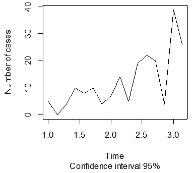
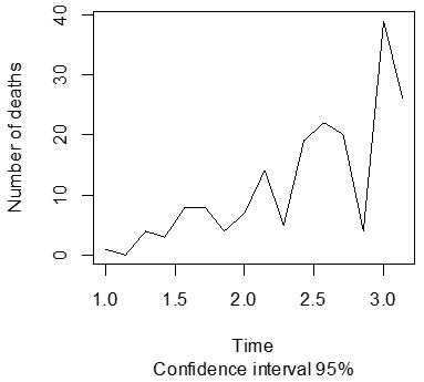
3.7 Forecast precision
Figures 2 and 3 below show a forecast of the number of COVID-19 cases and deaths for 12 periods.
From the graphs, it can be seen that there exists a constant rise in the figures of COVID-19 related cases alongside the death cases with a confidence interval of 95%.
Figure 2. Forecast for number of COVID-19 cases
Figure 3. Forecast for number of death
The surge of COVID-19 has crippled the health care system in Nigeria and other parts of the world. The need to model and study the incidence rate of COVID-19 cannot be overemphasized as it is pertinent for concrete decision making. There has been a sharp rise in the figures of COVID-19 cases and death as depicted by the time plot. The time plot of the number of cases and deaths shows an “S” shape which indicates the increase in the pandemic. A co-integration test was carried out which prompted the adoption of the Var model. A Vector Autoregressive model of lag 4 was adopted which was used to make a forecast on the number of cases and death. Moreover, an autocorrelation test and a test of heteroscedasticity were carried out where it was observed that there exists no autocorrelation at lag 3 and lag 4 and there exists no heteroscedasticity. A Jarque-Berra test of normality of the disturbances was done on the Vector Autoregressive model which indicates a departure from normality. However, this result can be ignored for a reasonable large sample size of at least 30 according to Ghasemi and Zahediasl [17]. The forecast also reveals an upward trend in the number of infections and death.
With respect to the above findings, the following recommendations have been made; (1) The government needs to put further measures in place to curtail the spread of the virus and aim towards flattening the curve, (2) an awareness should be created in order for individuals to be properly enlightened and get vaccinated.
This work is supported by the Covenant University Center for Research, Innovation and Discovery (CUCRID), Covenant University, Ota, Nigeria.
[1] World Health Organization. (www.who.int).
[2] Nigeria Center for Disease Control. (www.ncdc.gov.ng).
[3] Zeroual, A., Harrou, F., Dairi, A., Sun, Y. (2020). Deep learning methods for forecasting COVID-19 time series data: A Comparative study. Chaos, Solitons & Fractals, 140: 110121. https://doi.org/10.1016/j.chaos.2020.110121
[4] Petropoulos, F., Makridakis, S., Stylianou, N. (2020). COVID-19: Forecasting confirmed cases and deaths with a simple time series model. International Journal of Forecasting. https://doi.org/10.1016/j.ijforecast.2020.11.010
[5] Ribeiro, M., da Silva, R.G., Mariani, V.C., Coelho, L. (2020). Short-term forecasting COVID-19 cumulative confirmed cases: Perspectives for Brazil. Chaos, Solitons & Fractals, 135: 109853. https://doi.org/10.1016/j.chaos.2020.109853
[6] Nayak, S.R., Arora, V., Sinha, U., Poonia, R.C. (2021). A statistical analysis of COVID-19 using Gaussian and probabilistic model. Journal of Interdisciplinary Mathematics, 24(1): 19-32. https://doi.org/10.1080/09720502.2020.1833442
[7] de Figueiredo, A.M., Codina, A.D., Figueiredo, D.C.M.M., Saez, M., León, A.C. (2020). Impact of lockdown on COVID-19 incidence and mortality in China: An interrupted time series study. Bull World Health Organ. http://dx.doi.org/10.2471/BLT.20.256701
[8] Maleki, M., Mahmoudi, M.R., Heydari, M.H., Pho, K.H. (2020). Time series modelling to forecast the confirmed and recovered cases of COVID-19. Travel Medicine and Infectious Disease, 37: 101742. https://doi.org/10.1016/j.tmaid.2020.101742
[9] Dehkordi, A.H., Alizadeh, M., Derakhshan, P., Babazadeh, P., Jahandideh, A. (2020). Understanding epidemic data and statistics: A case study of COVID‐19. J Med Virol., 1-15. https://doi.org/10.1002/jmv.25885
[10] Chu, J. (2021). A statistical analysis of the novel coronavirus (COVID-19) in Italy and Spain. PLoS ONE, 16(3): e0249037. https://doi.org/10.1371/journal.pone.0249037
[11] Olusola-Makinde, O.O., Makinde, O.S. (2021). COVID-19 incidence and mortality in Nigeria: Gender based analysis. Peer J., 9: e10613. https://doi.org/10.7717/peerj.10613
[12] Tandon, H., Ranjan, P., Chakraborty, T., Suhag, V. (2020). Coronavirus (COVID-19): ARIMA based time series analysis to forecast near future. https://arxiv.org/abs/2004.07859.
[13] Juselius, K. (2007). Cointegration analysis of climate change. An exposition. Department of Economics, University of Copenhagen. https://citeseerx.ist.psu.edu/viewdoc/download?doi=10.1.1.407.8434&rep=rep1&type=pdf.
[14] Tsay, R.S. (2005). Analysis of Financial Time Series. John Wiley and Sons.
[15] Johansen, S. (1988). Statistical analysis of cointegration vectors. Journal of Economic Dynamics and Control, 12(2-3): 231-254. https://doi.org/10.1016/0165-1889(88)90041-3
[16] Box, G.E.P., Pierce, D.A. (1970). Distribution of residual correlations in autoregressive-integrated moving average time series models. Journal of the American Statistical Association, 65: 1509-1526. https://doi.org/10.1080/01621459.1970.10481180
[17] Ghasemi, A., Zahediasl, S. (2012). Normality tests for statistical analysis: A guide for non-statisticians. International Journal of Endocrinology and Metabolism, 10(2): 486. https://dx.doi.org/10.5812/ijem.3505