Bourhan Tashtoush* | Karima Megdouli | Towhid Gholizadeh | Elhadi Dekam
© 2021 IIETA. This article is published by IIETA and is licensed under the CC BY 4.0 license (http://creativecommons.org/licenses/by/4.0/).
OPEN ACCESS
To reduce fossil fuel consumption and its polluted environmental impact, a new enhanced waste heat recovery system operated by hot chimney flue gases from a cement plant is designed, analyzed, and evaluated. The configuration of the system is competitive and innovative. It is designed to be capable of producing space air cooling and electricity generation, simultaneously. Three temperature levels in the proposed cycle are considered, and a detailed mathematical model is developed with energy, exergy, and economic aspects are considered to achieve the best performance of the system. Computer FORTRAN subroutines are developed and run for simulation of several scenarios. A comprehensive parametric investigation and thermo-economic analysis are conducted and presented. It was found that the optimistic recovery system can achieve a refrigeration load coverage of 300 kW, while the energy and exergy efficiencies are 36.23% and 29.41%, respectively. The anticipated system seems to be optimistic knowing the cost of the product is estimated to be $45.97 per GJ.
energy, exergy, exergoeconomic, triple-evaporator, waste recovery systems
Industrial energy consumption constitutes more than 30% of the produced energy, and carbon dioxide production accounts for more than 5%. The cement production industry consumes a large portion of this energy, which attracted the attention of researchers to reduce the amount of energy consumed and mitigate carbon dioxide emissions. The creation of innovative solutions to supply the increase in demand for energy sustainably and cleanly to reduce environmental impact has been the focus of the research community for decades [1-3]. Different heat utilization methods were investigated to improve the system; energy efficiency [4-6].
The global warming process is a type of climate change that humanity has not yet overcome. Therefore, it is necessary to find out an ecological alternative that replaces conventional fuels, offers better performance, and achieves sustainability [7-10]. Renewable energy sources, waste material sources, and waste heat may be desirable choices to serve such issues. In fact, the recovery of industrial exhaust flue gases waste heat can be invested not only to generate electricity or heat water or gain a refrigerated capacity, but also to reduce exhaust toxic emissions, and therefore, reduce the pollution of the environment [10, 11].
It is important to improve the system’s energy efficiency in the manufacturing industry and reduce its dependability on fossil fuels since it consumes a large portion of worldwide energy [12, 13]. Experimental works were conducted on combined power cycles with the utilization of waste energy [14, 15]. This could be achieved by either enhancing the energy efficiency or increasing the use of renewable energies and waste heat [16-18]. The smart usage of renewable energies is the focus of many researchers to mitigate carbon dioxide and greenhouse emissions and reduce the impact on the environment. Many attempts had been made to design new sustainable systems and thermal cycles with better thermal efficiency [19-21].
Several research works have been done to study the performance of recovery-based systems employing waste heat from industrial plants and converted it into work, power, and cooling without supplying any additional fuel and with zero associated CO2 emissions. A thermo-economic analysis of a combined inverted Brayton/Organic Rankine cycle to utilize waste heat to generate mechanical power was presented [22]. The authors performed an optimization of the cycle and examined the performance of several working fluids. The organic Rankine cycle is known as the most promising potential technology in the application of heat recovery achievements in many theoretical and experimental research [23]. Combined power and cold generation cycles using a solar parabolic trough system were proposed and investigated [24]. They have studied the effects of the evaporation pressure and condensation temperature on the thermal efficiency of the introduced system.
An energy-saving scheme to recover the waste heat from vehicles by the integration of an ORC was introduced [25]. A multi-objective optimization model was developed to analyze the cycle performance and economy with different refrigerants. The utilization of the waste heat in a cement plant was studied and the results showed a great potential of recovering the wasted heat [26]. Thermo-economic assessments of a multipurpose energy system, which produces cooling and/or heating processes while it generates power was conducted [27, 28]. The results showed that the system is profitable and can save more than 30% of fuel. A new system that works with carbon dioxide was introduced and run by employing the waste heat accompanied the exhaust gas from a dual-fuel engine [29]. Their results indicate that the studied system could work efficiently based on the energy and economic points of view. A study of a modified ORC with solar energy as the energy source was also presented [30].
An environmental and thermo-economic analysis was presented and optimization of the ORC to improve its performance was made [31]. A new system, of transcritical carbon dioxide refrigeration cycle that is operated by waste heat was proposed [32]. The results confirmed an improvement in the energy and exergoeconomic efficiencies of the entire system.
Recently, ejector devices have been extensively studied employing both methods; computer simulation and mechanical laboratory, regarding their advantages, including easy to operate, require less maintenance with zero mechanical power required [33]. In this regard, the new system for the cooling process and power generation by the combination of the ORC with an ejector refrigeration cycle was proposed [34]. In the literature, ejectors are very well established and implemented in many applications in refrigeration technology [35-38].
A new system of two ejectors between three evaporators to have three levels of cooling pressures using the concept of throttling pressure drop was presented [39]. The main ejector was fed by the overall mixed stream, and the ejectors’ performance criteria depended on the operating state of the remaining two ejectors. To some extent, this seems to be complicated, and it was more difficult to control.
Referring to the conducted literature survey, one could conclude that the presented cement plant heat recovery cycle configuration, which is powered by the desired waste heat recovery system, has little trace in the published research work and it could be a very unique modern research point. The desired energy recovery system is an essential plan for strategical energy management in the industrial section. In the present work, a cement plant, with an exhaust flue gas temperature of 150°C, and a daily production capacity of 6.1 thousand tons clinker is considered. In this plant, the clinker calcination process consumes approximately 90% of the total energy as thermal energy. As a result of the total thermal energy consumed in the clinker calcination process, over 35% of the thermal energy is dissipated as waste heat to the environment without benefit. Therefore, a large amount of energy is wasted, and the heat pollution in the workplace is prominent and serious. The present work proposes a new system that is a valuable solution for the heat recovery project of the exhaust gases from the cement factory. This modern system is effectively safe for environmental issues through the prevention of high-temperature toxic flue gases entering the atmosphere contributing to global warming phenomena and acid rains. Due to the choking phenomenon of the ejector, a limited flow rate of the refrigerant could pass through. At this point, only part of the waste heat can be utilized. To maximize the amount of waste hat utilization, three ejectors connected in parallel are suggested in the new design. The new proposed system operates with 3×3 device sets, 3 ejectors, condensers, and evaporators, to provide a refrigeration capacity and generate electricity.
The main concept of the desired cycle provides an easier setting process for designers since each ejector performance has a weak function on the operating conditions of the other ejector. The most distinctive feature is that the current model is run by waste heat recovery from the cement plant. A comparative evaluation has been adjusted where the configuration setup and mathematical models are validated based on the published research cycle characteristics. The new thermal cycle is constructed concerning three different temperature levels. The thermodynamic analysis is accomplished in terms of energy and exergy principles, and exergoeconomic modeling is applied to distinguish the unit cost of products. Finally, a parametric study is conducted to demonstrate the sensitivity of the key parameters.
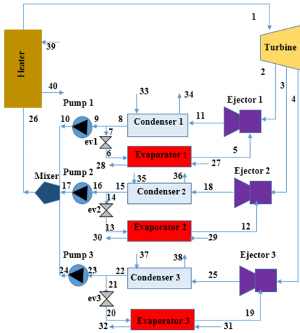
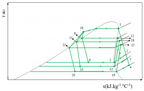
Figure 1 shows a schematic diagram for the proposed thermal recovery cycle. The main units of the cycle are a heat exchanger heater, a turbine coupled to an electrical generator, three space air cooling-based condensers, three refrigerant expansion valves, three refrigerant evaporators, three liquid pumps, and three ejector devices. Here, the heat exchanger heater exchanges heat with the plant chimney flue gases. Referring to the T-s diagram, Figure 2, the working fluid is heated in the heat exchanger plant by the waste exhaust heat, as mentioned above. Here, in each condenser, the superheated refrigerant vapor is condensed, due to the rejection of heat to the surroundings. This condensate is to be a saturated refrigerant liquid, which is diverted into two branches; one to the corresponding pump and the other to the corresponding expansion valves where the flows are throttled generating pressure drops at constant enthalpies. The outcome flow from the expansion valves goes into the evaporators as saturated vapor states.
Figure 1. A schematic diagram of the new cycle
Figure 2. The T-s diagram of the new cycle
Here, the evaporators provide cooling refrigerating capacity. The turbine exhaust flows through the ejectors and thus drawing the minor flows from the evaporators. In the ejectors, the mechanical energy is converted into kinetic energy. The pumps work on the three saturated liquid refrigerant lines which are to be in a compressed liquid state. These three sub-cooled streams are mixed, and the outflow is redirected to the heat exchanger heater to elevate its temperature to become saturated vapor at the highest pressure in the cycle. This liquid refrigerant flows with high temperature and pressure directed to the entrance of the turbine.
The cycle thermodynamic performance is evaluated by a thorough exergetic and energetic analysis of every component in the cycle. Economic and exergoeconomic analyses are also carried out to evaluate the feasibility of the proposed cycle. The conservation of energy and the 2nd law principles are applied to derive the system’s governing equations. In this work the following assumptions are made: steady-state flow, pressure drops are neglected except along ejectors, isentropic flow through the expansion valves, the refrigerant exits the condenser and evaporator at the saturated state and the Turbine and Pumps operate at given isentropic efficiencies. The thermodynamic parameters and system specifications are presented in Table 1.
Table 1. Thermodynamic system parameters
|
Parameters |
Value |
|
Reference state temperature, T0 |
20°C |
|
Reference state pressure, P0 |
1.01 bar |
|
Evaporator temperature 1 |
2°C |
|
Evaporator temperature 2 |
5°C |
|
Evaporator temperature 3 |
7°C |
|
Heater temperature |
130°C |
|
The expansion ratio of the turbine, BB1= p1/p2 |
3.5 |
|
The expansion ratio of the turbine, BB2=p1/p3 |
4 |
|
The expansion ratio of the turbine, BB3=p1/p4 |
4.5 |
|
The area ratio of the ejector, Φ |
6.8 |
|
Evaporator 1 cooling capacity |
100 kW |
|
Evaporator 2 cooling capacity |
100 kW |
|
Evaporator 3 cooling capacity |
100 kW |
|
Isentropic efficiency of the turbine, $\eta_{\text {tur }}$ |
0.9 |
|
Isentropic efficiency of the pump, $\eta_{p u}$ |
0.8 |
3.1 Thermal energy analysis
According to the conservation principles, the basic governing equations are derived for the steady-state flow processes. Here, the common continuity and energy equations can be written as follows:
$\sum_{i=1}^{m} \dot{m}_{i n}-\sum_{i=1}^{m} \dot{m}_{o u t}=0$ (1)
$\sum_{i=1}^{m}(\dot{m} h)_{i n}-\sum_{i=1}^{m}(\dot{m} h)_{o u t}+\sum_{i=1}^{m} \dot{Q}_{\text {in }}-\sum_{i=1}^{m} \dot{Q}_{\text {out }}+\dot{W}=0$ (2)
where, m is the number of entries or exists at the joint point.
Referring to the cycle, the ratio of the refrigerant mass flow entrained from the evaporator, ($\dot{m}_{s}$) to the refrigerant mass flow rate flowing out of the turbine, ($\dot{m}_{p}$) is defined as the entertainment ratio. This ratio has a significant effect on the ERC performance. This ratio can take the following form:
$U=\frac{\dot{m}_{s}}{\dot{m}_{p}}$ (3)
3.2 Exergy analysis
The above mathematical model of the first law of thermodynamics allows the calculation of the destructions and losses of the exergy that occurs at each component of the recovery cycle. The rate of the total exergy related to the system ($\dot{E}_{\text {total }}$) constitutes of the kinetic energy, physical, chemical, and potential exergy rates [40]. This can be presented as:
$\dot{E}_{\text {total }}=\dot{E}_{p h}+\dot{E}_{k n}+\dot{E}_{p t}+\dot{E}_{c h}$ (4)
The physical exergy rate is to be estimated as:
$\dot{E}_{p h}=\dot{m}\left[\left(h-h_{0}\right)-T_{0}\left(s-s_{0}\right)\right]$ (5)
where, h and s are the specific enthalpy and entropy of the refrigerant. The exergy balance of the system may be written as:
$\dot{E}_{F, t o t}=\dot{E}_{P, t o t}+\dot{E}_{D, t o t}+\dot{E}_{L, t o t}$ (6)
The system kth component’s exergy balance is:
$\dot{E}_{F, k}=\dot{E}_{P, k}+\dot{E}_{D, k}$ (7)
The system overall exergetic efficiency is given as:
$\eta_{e x}=\frac{\dot{E}_{P}}{\dot{E}_{F}}$ (8)
The mathematical relations that are derived based on the thermodynamic principles of the proposed system are given in Table 2.
3.3 Economic and exergoeconomic analysis
An economic evaluation of the proposed new hybrid cycle is obtained with the use of the Total Revenue Requirement (TRR) method. The formula for the calculation of the level zed total revenue requirement (TRRL) may be written as [40]:
$\mathrm{TRR}_{L}=\mathrm{CC}_{L}+\mathrm{FC}_{L}+\mathrm{OMC}_{L}$ (9)
With (CCL) is the levelized carrying charges, (FCL) is the levelized fuel cost, and $\mathrm{OMC}_{L}$ is the levelized operating and maintenance cost. Where:
$\mathrm{CC}_{L}=\mathrm{TCI}* \mathrm{CRF}$ (10)
$F C_{L}=F C_{0} * \frac{k_{F C}\left(1-\left(k_{F C}\right)^{n}\right)}{\left(1-k_{F C}\right)} * C R F$ (11)
$O M C_{L}=O M C_{0} * \frac{k_{O M C}\left(1-\left(k_{O M C}\quad
\right)^{n}
\right)}{\left(1-k_{O M C}\quad
\right)} * C R F$ (12)
CRF is the capital recovery factor and could be presented as follows:
$C R F=\frac{i(i+1)^{n}}{(1+i)^{n}-1}$ (13)
The capital recovery factor is defined as the ratio used to calculate the present value of a series of equal annual cash payments. These payments can be made at a regular interval of time, and are commonly known as annuities. In this case, n is equal to the number of years, and formula (13) gives the present value in terms of the number of years and i the interest rate.
$k=\frac{1+r}{1+i_{e f f}}$ (14)
where, $i_{e f f}$ and r are the effective and inflation interest rates, respectively.
TCI: The total capital investment.
n: The estimated number of years that represents the economic lifetime of the plant.
Table 2. Thermodynamic relations for the cycle components
|
Component |
Energy balances equations |
Exergy balance equations |
|
Evaporator 1 |
$\dot{Q}_{\text {eva1 }}=\dot{m}_{5} *\left(h_{5}-h_{6}\right)=\dot{m}_{27} *\left(h_{27}-h_{28}\right)$ |
$\dot{E} x_{D, \text { eva } 1}$ $=\left(\dot{E} x_{6}-\dot{E} x_{5}\right)$ $-\left(\dot{E} x_{28}-\dot{E} x_{27}\right)$ |
|
Evaporator 2 |
$\dot{Q}_{\text {eva } 2}=\dot{m}_{12} *\left(h_{12}-h_{13}\right)=\dot{m}_{29} *\left(h_{29}-h_{30}\right)$ |
$\dot{E} x_{D, e v a 2}$ $=\left(\dot{E} x_{13}-\dot{E} x_{12}\right)$ $-\left(\dot{E} x_{30}-\dot{E} x_{29}\right)$ |
|
Evaporator 3 |
$\dot{Q}_{\text {eva3 }}=\dot{m}_{19} *\left(h_{19}-h_{20}\right)=\dot{m}_{31} *\left(h_{31}-h_{32}\right)$ |
$\dot{E} x_{D, e v a 3}$ $=\left(\dot{E} x_{20}-\dot{E} x_{19}\right)$ $-\left(\dot{E} x_{32}-\dot{E} x_{30}\right)$ |
|
Condenser 1 |
$\dot{Q}_{\text {cond } 1}=\dot{m}_{8} *\left(h_{11}-h_{8}\right)=\dot{m}_{33} *\left(h_{34}-h_{33}\right)$ |
$\dot{E} x_{D, c o n d 1}$ $=\left(\dot{E} x_{11}-\dot{E} x_{8}\right)$ $-\left(\dot{E} x_{34}-\dot{E} x_{33}\right)$ |
|
Condenser 2 |
$\dot{Q}_{\text {cond } 2}=\dot{m}_{15} *\left(h_{18}-h_{15}\right)=\dot{m}_{35} *\left(h_{36}-h_{35}\right)$ |
$\dot{E} x_{D, \text { cond } 2}$ $=\left(\dot{E} x_{18}-\dot{E} x_{15}\right)$ $-\left(\dot{E} x_{36}-\dot{E} x_{35}\right)$ |
|
Condenser 3 |
$\dot{Q}_{\text {cond3 }}=\dot{m}_{22} *\left(h_{25}-h_{22}\right)=\dot{m}_{37} *\left(h_{38}-h_{37}\right)$ |
$\dot{E} x_{D, c o n d 3}$ $=\left(\dot{E} x_{25}-\dot{E} x_{22}\right)$ $-\left(\dot{E} x_{38}-\dot{E} x_{37}\right)$ |
|
Expansion valve 1 |
$h_{6}=h_{7}$ |
$\dot{E} x_{D, e v 1}=\dot{E} x_{7}-\dot{E} x_{6}$ |
|
Expansion valve 2 |
$h_{13}=h_{14}$ |
$\dot{E} x_{D, e v 2}=\dot{E} x_{14}-\dot{E} x_{13}$ |
|
Expansion valve 3 |
$h_{20}=h_{21}$ |
$\dot{E} x_{D, e v 3}=\dot{E} x_{20}-\dot{E} x_{21}$ |
|
Ejector 1 |
$\dot{m}_{11} * h_{11}=\dot{m}_{2} * h_{2}+\dot{m}_{5} * h_{5}$ |
$\dot{E} x_{D, e j 1}$ $=\dot{E} x_{2}+\dot{E} x_{5}-\dot{E} x_{11}$ |
|
Ejector 2 |
$\dot{m}_{18} * h_{18}=\dot{m}_{3} * h_{3}+\dot{m}_{12} * h_{12}$ |
$\dot{E} x_{D, e j 2}$ $=\dot{E} x_{3}+\dot{E} x_{12}-\dot{E} x_{18}$ |
|
Ejector 3 |
$\dot{m}_{25} * h_{25}=\dot{m}_{4} * h_{4}+\dot{m}_{19} * h_{19}$ |
$\dot{E} x_{D, e j 3}$ $=\dot{E} x_{4}+\dot{E} x_{19}-\dot{E} x_{25}$ |
|
Pump 1 |
$\dot{W}_{p u 1}=\dot{m}_{10} *\left(h_{10}-h_{9}\right)$; $\eta_{p u 1}=\frac{h_{10 s}-h_{9}}{h_{10}-h_{9}}$ |
$\dot{E} x_{D, p u 1}$ $=\dot{W}_{p u 1}-\left(\dot{E} x_{10}-\dot{E} x_{9}\right)$ |
|
Pump 2 |
$\dot{W}_{p u 2}=\dot{m}_{17} *\left(h_{17}-h_{16}\right) ;$ $\eta_{p u 2}=\frac{h_{17 s}-h_{16}}{h_{17}-h_{16}}$ |
$\dot{E} x_{D, p u 2}$ $=\dot{W}_{p u 2}-\left(\dot{E} x_{17}-\dot{E} x_{16}\right)$ |
|
Pump 3 |
$\dot{W}_{p u 3}=\dot{m}_{24} *\left(h_{24}-h_{23}\right) ;$ $\eta_{\text {puз }}=\frac{h_{24 s}-h_{23}}{h_{24}-h_{23}}$ |
$\dot{E} x_{D, p u 3}$ $=\dot{W}_{p u 3}-\left(\dot{E} x_{24}-\dot{E} x_{23}\right)$ |
|
Turbine |
$\dot{W}_{t u r}=\dot{m}_{1} *\left(h_{1}-h_{2}\right)+\left(\dot{m}_{1}-\dot{m}_{2}\right) *\left(h_{2}-h_{3}\right)+$ $\left(\dot{m}_{1}-\dot{m}_{2}-\dot{m}_{3}\right) *\left(h_{3}-h_{4}\right)$ $\eta_{t u r}=\frac{h_{1}-h_{2}}{h_{1}-h_{2 s}}=\frac{h_{2}-h_{3}}{h_{2}-h_{3 s}}=\frac{h_{3}-h_{4}}{h_{3}-h_{4 s}}$ |
$\dot{E} x_{D, t u r}=\dot{E} x_{1}-\dot{E} x_{2}-\dot{E} x_{3}-\dot{E} x_{4}-\dot{W}_{t u r}$ |
|
Heater |
$\dot{Q}_{H E}=\dot{m}_{1} *\left(h_{1}-h_{26}\right)=\dot{m}_{39} *\left(h_{39}-h_{40}\right)$ |
$\dot{E} x_{D, H E}=\left(\dot{E} x_{39}-\dot{E} x_{40}\right)-\left(\dot{E} x_{1}-\dot{E} x_{26}\right)$ |
|
mixer |
$\dot{m}_{26} * h_{26}=\left(\dot{m}_{10} * h_{10}\right)+\left(\dot{m}_{17} * h_{17}\right)+$ $\left(\dot{m}_{24} * h_{24}\right)$; $\dot{m}_{26}=\dot{m}_{10}+\dot{m}_{17}+\dot{m}_{24}$ |
$\dot{E} x_{D, \operatorname{mix}}=\dot{E} x_{10}+\dot{E} x_{17}+\dot{E} x_{24}-\dot{E} x_{26}$ |
The subscript “0” refers to the beginning of the first year.
For simplification, k is assumed to be as follows:
$k=k_{F C}=k_{O M C}$ (15)
The whole recovery system should be operated by the actual waste heat. Therefore, the fuel cost is assumed to be zero, and the levelized fuel cost, $F C_{L}$ = 0. TCI is assumed to be a function of the total cost of the purchased equipment (PECtotal) of the plant. For the new proposed cycle, TCI can be expressed as follows [41]:
$T C I=6.32 * P E C_{\text {total }}$ (16)
It is assumed that the plant has an economic lifetime of n equals to 20 years, $i_{\text {eff }}$ is 10%, and r is 2.5% [41].
The cost rate of product $\dot{C}_{P, k}$ for the kth component could be written as [42]:
$\dot{C}_{P, k}=\dot{C}_{F, k}+\dot{Z}_{k}$ (17)
where, $\dot{C}_{F, k}$ is the fuel cost rate, and $\dot{Z}_{k}$ is the summation of the cost rates of the capital investment $\dot{Z}_{k}^{C I}$ and the operating and maintenance expenses $\dot{Z}_{k}^{O M}$ of the k component. The value of $\dot{Z}_{k}$ is:
$\dot{Z}_{k}=\dot{Z}_{k}^{C I}+\dot{Z}_{k}^{O M}$ (18)
$\dot{Z}_{k}^{C I}=\frac{C C_{L}}{\tau} * \frac{P E C_{k}}{P E C_{t o t a l}}$ (19)
$\dot{Z}_{k}^{O M}=\frac{O M C_{L}}{\tau} * \frac{P E C_{k}}{P E C_{\text {total }}}$ (20)
where, τ is the number of working hours per year. It is assumed to be 8000 hr/year. Table 3 listed the cost balance and auxiliary equations.
Table 3. Cost term equations for each component in the cycle
|
Component |
Cost balance equation |
Auxiliary equation |
Cost equation ($) [42, 43] |
|
Evaporator1 |
$\dot{C}_{5}+\dot{C}_{28}=\dot{C}_{27}+\dot{C}_{6}+\dot{Z}_{\text {eva1 }}$ |
$c_{27}=0$, $c_{5}=c_{6}$ |
$P E C_{\text {eva } 1}=6000 *\left(\frac{A_{\text {eva1 }}}{100}\right)^{0.7}$ |
|
Evaporator2 |
$\dot{C}_{12}+\dot{C}_{30}=\dot{C}_{29}+\dot{C}_{13}+\dot{Z}_{\text {eva } 2}$ |
$c_{29}=0$, $c_{12}=c_{13}$ |
$P E C_{e v a 2}=6000 *\left(\frac{A_{e v a 2}}{100}\right)^{0.7}$ |
|
Evaporator3 |
$\dot{C}_{19}+\dot{C}_{32}=\dot{C}_{20}+\dot{C}_{31}+\dot{Z}_{\text {eva3 }}$ |
$c_{31}=0$, $c_{19}=c_{20}$ |
$P E C_{\text {eva3 }}=6000 *\left(\frac{A_{\text {eva3 }}}{100}\right)^{0.7}$ |
|
Condenser1 |
$\dot{C}_{8}+\dot{C}_{34}=\dot{C}_{11}+\dot{C}_{33}+\dot{Z}_{\text {cond } 1}$ |
$c_{33}=0, c_{11}=c_{8}$ |
$P E C_{\text {cond } 1}=1773 * m_{8}$ |
|
Condenser2 |
$\dot{C}_{15}+\dot{C}_{36}=\dot{C}_{18}+\dot{C}_{35}+\dot{Z}_{\text {cond } 2}$ |
$c_{35}=0, c_{18}=c_{15}$ |
$P E C_{\text {cond } 2}=1773 * m_{15}$ |
|
Condenser3 |
$\dot{C}_{22}+\dot{C}_{38}=\dot{C}_{25}+\dot{C}_{37}+\dot{Z}_{\text {cond } 3}$ |
$c_{37}=0, c_{22}=c_{25}$ |
$P E C_{\text {cond } 3}=1773 * m_{22}$ |
|
Expansion valve 1 |
$\dot{C}_{6}=\dot{C}_{7}+\dot{Z}_{e v 1}$ |
- |
$P E C_{e v 1}=100$ |
|
Expansion valve 2 |
$\dot{C}_{13}=\dot{C}_{14}+\dot{Z}_{e v 2}$ |
- |
$P E C_{e v 2}=100$ |
|
Expansion valve 3 |
$\dot{C}_{20}=\dot{C}_{21}+\dot{Z}_{e v 3}$ |
- |
$P E C_{e v 3}=100$ |
|
Ejector 1 |
$\dot{C}_{11}=\dot{C}_{2}+\dot{C}_{5}+\dot{Z}_{e j 1}$ |
- |
$P E C_{e j 1}=0$ |
|
Ejector 2 |
$\dot{C}_{18}=\dot{C}_{3}+\dot{C}_{12}+\dot{Z}_{e j 2}$ |
- |
$P E C_{e j 2}=0$ |
|
Ejector 3 |
$\dot{C}_{25}=\dot{C}_{4}+\dot{C}_{19}+\dot{Z}_{e j 3}$ |
- |
$P E C_{e j 3}=0$ |
|
Pump 1 |
$\dot{C}_{10}=\dot{C}_{9}+\dot{C}_{w, p u 1}+\dot{Z}_{p u 1}$ |
- |
$P E C_{p u 1}=3540 * W_{p u 1}^{0.71}$ |
|
Pump 2 |
$\dot{C}_{17}=\dot{C}_{16}+\dot{C}_{w, p u 2}+\dot{Z}_{p u 2}$ |
- |
$P E C_{p u 2}=3540 * W_{p u 2}^{0.71}$ |
|
Pump 3 |
$\dot{C}_{24}=\dot{C}_{23}+\dot{C}_{w, p u 3}+\dot{Z}_{p u 3}$ |
- |
$P E C_{p u 3}=3540 * W_{p u 3}^{0.71}$ |
|
Division point 1 |
- |
$C_{9}=C_{7}$ |
|
|
Division point 2 |
- |
$c_{15}=c_{14}$ $c_{15}=c_{16}$ |
- |
|
Division point 3 |
- |
$c_{22}=c_{23}$ $c_{22}=c_{21}$ |
- |
|
Turbine |
$\dot{C}_{1}+\dot{Z}_{t u r}=\dot{C}_{2}+\dot{C}_{3}+\dot{C}_{4}+\dot{C}_{w, t u r}$ |
$c_{1}=c_{2} ; c_{1}=c_{3}$; $c_{1}=c_{4}$ |
$P E C_{t u r}=6000 * \dot{W}_{t u r}^{0.7}$ |
|
Heater |
$\dot{C}_{40}+\dot{C}_{1}=\dot{C}_{39}+\dot{C}_{26}+\dot{Z}_{H E}$ |
$c_{40}=c_{39}$ $c_{39}=0$ |
$P E C_{H E}=309.143 * A_{H E}+231.915$ |
|
Mixer |
$\dot{C}_{26}=\dot{C}_{10}+\dot{C}_{17}+\dot{C}_{24}+\dot{Z}_{\operatorname{mix}}$ |
- |
$P E C_{\operatorname{mix}}=0$ |
The value of the final cost of the product, $C_{p, \text { total }}$ is:
$c_{p, t o t a l}=\frac{\dot{C}_{P, t o t a l}+\dot{C}_{L, t o t a l}}{\dot{E}_{P, \text { total }}}$ (21)
The total exergoeconomic factor is defined as follows:
$f_{\text {total }}=\frac{\dot{Z}_{\text {total }}}{\dot{Z}_{\text {total }}\quad
+\dot{C}_{D, \text { total }}}$ (22)
where,
$\dot{C}_{D, \text { total }}=c_{F, t o_{t a l}} \sum \dot{E}_{k, D}$ (23)
4.1 Model validation and results comparison
A FORTRAN computer code is developed to simulate the recovery system cycle. To validate the output results and show the accuracy of the developed code, different results related to several studies from the literature are selected for comparison purposes. The present results obtained are validated with the experimental data reported in the literature [44]. This validation was carried out with R141b as a working fluid and with an ejector geometry size of d = 2.64 mm and D1 = 4.5 mm. Referring to Table 4, the validation indicates a good agreement with such published data.
Table 4. Ejector modeling validation of the present work with experimental published data [44]
|
$\boldsymbol{T}_{p f}$ (°C) |
$T_{s f}$ (°C) |
$\boldsymbol{T}_{\text {cond }}$ (°C) |
Uexp [38] |
Ucalc |
|
78 |
8 |
32.5 |
0.3257 |
0.3108 |
|
84 |
8 |
35.5 |
0.288 |
0.2867 |
|
90 |
8 |
38.9 |
0.2246 |
0.2226 |
|
95 |
8 |
42.1 |
0.1859 |
0.1858 |
|
84 |
12 |
36 |
0.3398 |
0.3532 |
|
90 |
12 |
39.5 |
0.2946 |
0.2921 |
|
95 |
12 |
42.5 |
0.235 |
0.2449 |
|
Fluid: R141b; $\varphi=A_{e 3} / A_{t}=6.44$ |
||||
Table 5. Comparison of the present and published results
|
Performance parameters |
Unit |
Published results, [39] |
Current work |
|
|
The BTECCP cycle |
The RTECCP cycle |
|||
|
Cooling load ($\dot{Q}_{\text {eva,total }}$) |
kW |
98.5 |
96.7 |
239.8 |
|
Net electricity ($\dot{W}_{\text {net }}$) |
kW |
53.4 |
60.7 |
16.6 |
|
Thermal efficiency |
% |
34.1 |
35.3 |
37.5 |
|
Exergy efficiency |
% |
33.6 |
37.9 |
25.4 |
|
The total sum unit cost of the product |
$\$ . G J^{-1}$ |
362.5 |
371.1 |
108.1 |
|
Fluid: Butene; THE= 129.25 (°C); Teva1= -30.95 (°C); Teva2=4.85 (°C); Teva3= 8.85 (°C) |
||||
Table 6. Cycle state properties
|
Point |
T(K) |
P(MPa) |
h(kJ.kg-1) |
s(kJ.kg-1.K-1) |
$\dot{m}$ (kg.s-1) |
$\dot{\boldsymbol{E}}$ (kW) |
$\dot{C}\left(\$ . h^{-1}\right)$ |
$c\left(\$ \cdot G J^{-1}\right)$ |
|
1 |
403.1 |
2344.2 |
487.7 |
1.8 |
4.1 |
669.7 |
48.4 |
20.1 |
|
2 |
355.9 |
669.8 |
468.01 |
1.8 |
2.0 |
281.8 |
20.4 |
20.1 |
|
3 |
353.91 |
586.1 |
467.7 |
1.8 |
1.2 |
171.9 |
12.4 |
20.1 |
|
4 |
352.5 |
520.9 |
467.66 |
1.8 |
0.9 |
122.3 |
8.84 |
20.1 |
|
5 |
275.1 |
57.95 |
405.9 |
1.7 |
0.6 |
57.2 |
7.3 |
35.1 |
|
6 |
275.1 |
57.95 |
235. |
1.1 |
0.6 |
63.7 |
8.2 |
35.1 |
|
7 |
300.1 |
159.3 |
235. |
1.1 |
0.6 |
64.6 |
8.2 |
35.1 |
|
8 |
300.1 |
159.3 |
235. |
1.1 |
2.6 |
282.2 |
26.1 |
25.7 |
|
9 |
300.1 |
159.3 |
235. |
1.1 |
2.0 |
217.7 |
27.5 |
35.1 |
|
10 |
301.2 |
2344.2 |
237.1 |
1.1 |
2.0 |
220.9 |
28.2 |
35.4 |
|
11 |
330.9 |
159.3 |
453.8 |
1.8 |
2.6 |
298.8 |
27.7 |
25.7 |
|
12 |
278.1 |
66.2 |
408.1 |
1.7 |
0.6 |
56.9 |
4.8 |
23.4 |
|
13 |
278.1 |
66.2 |
232.5 |
1.1 |
0.6 |
62.3 |
5.3 |
23.4 |
|
14 |
298.1 |
148.2 |
232.5 |
1.1 |
0.6 |
62.8 |
5.3 |
23.2 |
|
15 |
298.1 |
148.2 |
232.5 |
1.1 |
1.8 |
197.6 |
16.5 |
23.2 |
|
16 |
298.1 |
148.2 |
232.5 |
1.1 |
1.2 |
134.8 |
11.3 |
23.2 |
|
17 |
299.2 |
2344.2 |
234.5 |
1.114 |
1.2 |
136.8 |
11.7 |
23.8 |
|
18 |
325.4 |
148.2 |
448.7 |
1.835 |
1.8 |
206.1 |
17.2 |
23.2 |
|
19 |
280.1 |
72.22 |
409.6 |
1.748 |
0.6 |
56.5 |
4.7 |
23.1 |
|
20 |
280.1 |
72.2 |
230.4 |
1.109 |
0.6 |
61.2 |
5.1 |
23.1 |
|
21 |
296.6 |
140.0 |
230.4 |
1.106 |
0.6 |
61.6 |
5.1 |
23.0 |
|
22 |
296.6 |
140.0 |
230.4 |
1.1 |
1.4 |
158.7 |
13.1 |
23.0 |
|
23 |
296.6 |
140.0 |
230.4 |
1.106 |
0.9 |
97.2 |
8.1 |
23.0 |
|
24 |
297.7 |
2344.2 |
232.5 |
1.1 |
0.9 |
98.6 |
8.4 |
23.6 |
|
25 |
321.4 |
140.0 |
445.1 |
1.8 |
1.4 |
163.7 |
13.5 |
23.0 |
|
26 |
299.8 |
2344.2 |
235.3 |
1.1 |
4.1 |
456.3 |
48.3 |
29.4 |
|
27 |
285.1 |
101 |
411.4 |
3.8 |
19.9 |
2.2 |
0 |
0 |
|
28 |
280.1 |
101 |
406.3 |
3.8 |
19.9 |
5.9 |
0.9 |
41.3 |
|
29 |
288.1 |
101 |
414.4 |
3.9 |
19.9 |
0.8 |
0 |
0 |
|
30 |
283.1 |
101 |
409.3 |
3.8 |
19.9 |
3.4 |
0.5 |
39.8 |
|
31 |
290.1 |
101 |
416.4 |
3.8 |
19.9 |
0.2 |
0 |
0 |
|
32 |
285.1 |
101 |
411.4 |
3.8 |
19.9 |
2.2 |
0.4 |
54.5 |
|
33 |
293.1 |
101 |
84 |
0.3 |
27.0 |
0 |
0 |
0 |
|
34 |
298.1 |
101 |
104.7 |
0.4 |
27.0 |
4.7 |
1.6 |
98.0 |
|
35 |
293.1 |
101 |
84 |
0.3 |
30.9 |
0 |
0 |
0 |
|
36 |
296.1 |
101 |
96.5 |
0.3 |
30.9 |
1.9 |
0.8 |
111.5 |
|
37 |
293.1 |
101 |
84 |
0.3 |
50.3 |
0 |
0 |
0 |
|
38 |
294.6 |
101 |
90.1 |
0.3 |
50.3 |
0.7 |
0.5 |
178.0 |
|
39 |
413.1 |
101 |
540.6 |
4.2 |
50.7 |
994.6 |
0 |
0 |
|
40 |
393.1 |
101 |
520.3 |
4.2 |
50.7 |
714.3 |
0 |
0 |
Furthermore, a comparison is made to the published data [39] to evaluate the advantages of the present model over the previously published models. As shown in Table 5, the present model produces cooling capacity in the order of 2.5 times more than that was produced by Rostamzadeh et al. [39]. However, the desired present cycle generates about 70% less electricity than that was produced. The thermal efficiency of the new model is higher than that of the BTECCP and RTECCP cycles, approximately 10.28%, and 6.46%, respectively, while the exergy overall efficiency of the introduced cycle is lower than that of the BTECCP and RTECCP cycles, approximately, 24.3% and 32.83%, respectively. Regarding the economic analysis side, the total cost of the unit of the product for the running cycle reached \$108.1 per GJ, while the corresponding total cost for the BTECCP and RTECCP cycles are \$362.5 per GJ, and \$371.1 per GJ, respectively.
4.2 The cycle thermodynamic and economic results
The calculated values of the properties at each state point are introduced in Table 6, based on the conditions given in Table 1.
The cycle thermodynamic and economic performances are presented in Table 7.
Table 7. The cycle thermodynamic and economic performance
|
Parameter |
Value |
|
The net power rate (kW) |
72.55 |
|
The produced cooling rate (kW) |
300 |
|
Energy efficiency (%) |
36.23 |
|
Exergy efficiency (%) |
29.41 |
|
Exergy destruction rate [kW] |
192.32 |
|
$C_{p, t o t a l}$ [$.GJ-1] |
45.97 |
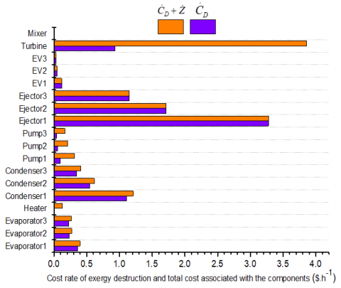
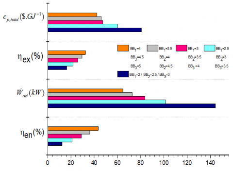
The results obtained from the exergoeconomic analysis, Figure 3, show that the cost of exergy destruction, $\dot{C}_{D}$, in the heater is zero, since the fuel, waste heat from the cement plant, is supposed to be free of charge, while it has the highest value within ejector 1. It should be noted that ejectors 2 and 3 also have the notable costs of exergy destruction. Ejectors need to be given more attention to sharing more in the upgrade of the overall cycle performance. More data and extra details are documented by Tashtoush et al. [16]. The total costs associated with each component are the sum of $\dot{C}_{D}+\dot{Z}$. The cost values for the turbine are quite remarkable mainly because of the contribution of the $\dot{Z}_{t u r}$.
4.3 Effects of heater temperature
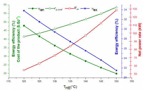
The variations of the thermal and exergy efficiencies, the system’s product cost, and the net power output as a function of the heater temperature are illustrated in Figure 4. Since the input energy into the turbine increases, the net power output increases as the heater temperature increases. An increase of 25% in the heater temperature resulted in a 160% increase in the net power output. The amount of heat input of the system, $\dot{Q}_{H E}$ increase with the increase in the heater temperature; therefore, the thermal and exergy efficiencies decrease. Furthermore, a 25% increase in the heater temperature would result in a 50% increase in the system total product cost, $c_{p, \text { total }}$.
Figure 3. The total and the exergy destruction cost rates, $\dot{\mathrm{C}}_{\mathrm{D}}$, and $\dot{\mathrm{C}}_{\mathrm{D}}+\dot{\mathrm{Z}}$
Figure 4. Effect of heater temperature on system performance
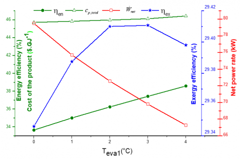
The Effect of the 1st Evaporator Temperature. The variation of different system parameters with the 1st evaporator temperature is illustrated in Figure 5. As the refrigerating capacity, $\dot{\boldsymbol{Q}}_{\text {eva1 }}$ is held constant, the primary mass flow rate of the first ejector decreases, which leads to an increase in the system energy efficiency and a decrease in the net power output. The trend of the exergy efficiency variation exhibits a maximum point at a value of 29.41% corresponding to an optimum evaporator temperature range of 2-3oC. finally, since there are no considerable cost changes in the variation of the 1st evaporator temperature, the system total product cost of the system is almost constant.
Figure 5. The effect of the 1st evaporator temperature on the system performance
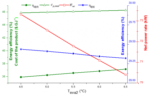
The Effect of the 2nd Evaporator Temperature. The effect of the variation of the 2nd evaporator temperature on the system performance is shown in Figure 6. It is noted that the most affected parameter by the variation of the evaporator temperature is the net power output. The exergy efficiency decreases relatively as the 2nd evaporator temperature increases. In the meantime, the thermal efficiency and the cost related to the cycle are increased with the increase of the 2nd evaporator temperature.
Figure 6. The effect of the 2nd evaporator temperature on the system performance
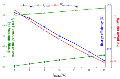
The Effects of the 3rd Evaporator Temperature. The effect of the 3rd evaporator temperature on the system performance is illustrated in Figure 7. Since the evaporator pressure increases as the temperature increases, a lower primary mass flow rate is needed to create the suction effect and entrain the adequate amount of refrigerant. The net power output and exergy efficiency decrease sharply as the evaporator temperature increase. The thermal energy efficiency and cost of the product moderately increase with the temperature. The energy efficiency is better once the temperature of the third evaporator is higher. From the exergoeconomic point of view, the decrease in the evaporator’s temperature will result in a decrease in the system's total product cost.
The Effect of Turbine Expansion Ratio. The effect of the turbine’s expansion ratios on the system performance parameters is shown in Figure 8. An increase in the thermal and exergetic efficiencies and a decrease in the net power output are noted as the expansion ratio increases. Besides, the system's total cost of the product decreases as the expansion ratio increases.
The study was done on the potential of a new design for a waste energy recovery system that is to be operated by cement plant exhaust hot flue gases in Tunisia, which is expected to contribute to sustainable development and cleaner production. The new system design leads to produce a cooling capacity and generate electricity, simultaneously, while implementing three working device sets at three temperature levels arranged in parallel. This cycle configuration is evaluated from the energy, exergetic, and exergoeconomic viewpoints, while a parametric study is accomplished.
The turbine has the highest total cost, among all components. The energy and exergy efficiencies and the cost of the product are 36.23%, 29.41%, and 45.97 \$.GJ-1, respectively. It’s found that the thermal efficiency can be increased by increasing the expansion ratio, evaporator temperature, or by decreasing the heater temperature. It was found that the exergy efficiency could be increased by the increase in the expansion ratio or the 1st evaporator temperature, or by the decrease in the heater temperature. While increasing the evaporation temperature, the cost of the product increases gradually. This recovery cycle is very attractive to apply in different industrial plants to achieve the share for sustainable, and efficient energy, and lower product costs.
Figure 7. The effect of the 3rd evaporator temperature variation on the system performance
Figure 8. The expansion ratio effect on system performance
|
Symbols |
|
|
c |
cost per unit of exergy [\$GJ-1] |
|
$\dot{C}$ |
Cost rate |
|
CRF |
capital recovery factor |
|
$\dot{E}$ |
exergy rate (kW) |
|
$\dot{E}_{D, t o t}$ |
total exergy destruction cost rate (kW) |
|
f |
exergoeconomic factor |
|
h |
specific enthalpy (kJ.kg-1) |
|
i |
interest rate |
|
LMTD |
logarithmic mean temperature difference (k) |
|
$\dot{m}$ |
mass flow rate (kg.s-1) |
|
N |
annual number of hours (hr) |
|
P |
pressure (MPa) |
|
$\dot{Q}$ |
heat transfer rate (kW) |
|
r |
relative cost difference |
|
s |
specific entropy (kJ.kg-1.k-1) |
|
T |
temperature (°C or k) |
|
$\dot{W}$ |
electrical power (kW) |
|
Z |
investment cost of components (\$) |
|
$\dot{Z}$ |
investment cost rate of components (\$/h) |
|
$\dot{Z}_{\text {tot }}$ |
total capital cost rate (\$/h) |
|
Abbreviations |
|
|
HE |
heater |
|
cond |
condenser |
|
eva |
evaporator |
|
ev |
expansion valve |
|
tur |
turbine |
|
Ej |
ejector |
|
tot |
total value |
|
pu |
pump |
|
Subscripts |
|
|
0 |
environmental stat |
|
1,2,3, |
cycle locations |
|
F |
fuel |
|
in |
inlet |
|
is |
isentropic |
|
k |
each component |
|
out |
outlet |
|
P |
product |
|
Greek Symbols |
|
|
η |
efficiency (%) |
[1] Zhang, W., Malek, A., Khajeh, M., Zhang, Y., Mortazavi, S.M., Vasel-Be-Hagh, A. (2019). A novel framework for integrated energy optimization of a cement plant: An industrial case study. Sustainable Energy Technologies and Assessments, 35: 245-256. https://doi.org/10.1016/j.seta.2019.06.001
[2] Ishak, S.A., Hashim, H. (2015). Low carbon measures for cement plant–a review. J Clean Prod., 103: 260-274. https://doi.org/10.1016/j.jclepro.2014.11.003
[3] Mohammadi, K., Khaledi, M., Saghafifar, M., Powell, K. (2020). Hybrid systems based on gas turbine combined cycle for trigeneration of power, cooling, and freshwater: A comparative techno-economic assessment. Sustainable Energy Technologies and Assessments, 37: 100632. https://doi.org/10.1016/j.seta.2020.100632
[4] Gianluca, V., Alessandro, V., Simone, S. (2019). Proposal of a thermally driven air compressor for waste heat recovery. Energy Convers Manage., 196: 1113-25. https://doi.org/10.1016/j.enconman.2019.06.072
[5] Giovanni, M., Maria, F. (2019). Supercritical CO2 power cycles for waste heat recovery: A systematic comparison between traditional and novel layouts with dual expansion. Energy Convers Manage, 197: 111777. https://doi.org/10.1016/j.enconman.2019.111777
[6] Woolley, E., Luo, Y., Simeone, A. (2018). Industrial waste heat recovery: A systematic approach. Sustainable Energy Technologies and Assessments, 29: 50-59. https://doi.org/10.1016/j.seta.2018.07.001
[7] Sorrell, S. (2015). Reducing energy demand: A review of issues, challenges and approaches. Renew Sustain Energy Rev., 47: 74-82. https://doi.org/10.1016/j.rser.2015.03.002
[8] Vallack, H., Timmis, A., Robinson, K., Sato, M. (2011). Technology innovation for energy intensive industry in the United Kingdom. York: Low Carbon Futures.
[9] Elakhdar, M., Landoulsi, H., Tashtoush, B., Nehdi, E., Kairouani, L. (2019). A combined thermal system of ejector refrigeration and Organic Rankine cycles for power generation using a solar parabolic trough. Energy Convers Manage., 199: 111947. https://doi.org/10.1016/j.enconman.2019.111947
[10] Dincer, I. (2000). Renewable energy and sustainable development: A crucial review. Renewable and Sustainable Energy Reviews, 4(2): 157-75. https://doi.org/10.1016/S1364-0321(99)00011-8
[11] Tashtoush, B., Younes, M.B. (2019). Comparative thermodynamic study of refrigerants to select the best environment-friendly refrigerant for use in a solar ejector cooling system. Arab J Sci Eng., 44: 1165-1184. https://doi.org/10.1007/s13369-018-3427-4
[12] Woolley, E., Luo, Y., Simeone, A. (2018). Industrial waste heat recovery: A systematic approach. Sustainable Energy Technologies and Assessments, 29: 50-59. https://doi.org/10.1016/j.seta.2018.07.001
[13] Megdouli, K., Tashtoush, B., Nahdi, E., Elakhdar, M., Kairouani, L., Mhimid, A. (2016). Thermodynamic analysis of a novel ejector cascade refrigeration cycles for freezing process applications and air-conditioning. International Journal of Refrigeration, 70: 108-118. https://doi.org/10.1016/j.ijrefrig.2016.06.029
[14] Yu, G.P., Shu, G.Q., Tian, H., Huo, Y.Z., Zhu, W.J. (2016). Experimental investigations on a cascaded steam-/organic-Rankine-cycle (RC/ORC) system for waste heat recovery (WHR) from diesel engine. Energy Conversion and Management, 129: 43-51. https://doi.org/10.1016/j.enconman.2016.10.010
[15] Remeli, M.F., Date, A., Orr, B., Ding, L.C., Singh, B., Nor Affandi, N.D., Akbarzadeh, A. (2016). Experimental investigation of combined heat recovery and power generation using a heat pipe assisted thermoelectric generator system. Energy Conversion and Management, 111: 147-157. https://doi.org/10.1016/j.enconman.2015.12.032
[16] Tashtoush, B.M., Al-Nimr, M.A., Khasawneh, M.A. (2017). Investigation of the use of nano-refrigerants to enhance the performance of an ejector refrigeration system. Appl Energy, 206: 1446-1463. https://doi.org/10.1016/j.apenergy.2017.09.117
[17] Tashtoush, B., Nayfeh, Y. (2020). Energy and economic analysis of a variable-geometry ejector in solar cooling systems for residential buildings. J Energy Storage, 27: 101061. https://doi.org/10.1016/j.est.2019.101061
[18] Megdouli, K., Sahli, H., Tashtoush, B., Nahdi, E., Kairouani, L. (2019). Theoretical research of the performance of a novel enhanced transcritical CO2 refrigeration cycle for power and cold generation. Energy Conversion and Management, 201: 112139. https://doi.org/10.1016/j.enconman.2019.112139
[19] Omer, G., Yavuz, A., Ahiska, R., Calisal, K. (2020). Smart thermoelectric waste heat generator: Design, simulation and cost analysis. Sustainable Energy Technologies and Assessments, 37: 100623. https://doi.org/10.1016/j.seta.2019.100623
[20] Emeksiz, C., Demirci, B. (2019). The determination of offshore wind energy potential of Turkey by using novelty hybrid site selection method. Sustainable Energy Technol Assess, 36: 1-21. https://doi.org/10.1016/j.seta.2019.100562
[21] Emeksiz, C., Cetin, T. (2019). In case study: Investigation of tower shadow disturbance and wind shear variations effects on energy production, wind speed and power characteristics. Sustainable Energy Technol Assess, 35: 148-59. https://doi.org/10.1016/j.seta.2019.07.004
[22] Abrosimov, K., Baccioli, A., Bischi, A. (2019). Techno-economic analysis of combined inverted Brayton/Organic Rankine cycle for high-temperature waste heat recovery. Energy Conversion and Management, 3: 100014. https://doi.org/10.1016/j.ecmx.2019.100014
[23] Hoang, A. (2018). Waste heat recovery from diesel engines based on Organic Rankine Cycle. Applied Energy, 231: 138-166. https://doi.org/10.1016/j.apenergy.2018.09.022
[24] Elakhdar, M., Landoulsi, H., Tashtoush, B., Nehdi, E., Kairouani, L. (2019). A combined thermal system of ejector refrigeration and Organic Rankine cycles for power generation using a solar parabolic trough. Energy Convers Manage., 199: 111947. https://doi.org/10.1016/j.enconman.2019.111947
[25] Imran, M., Haglind, F., Lemort, V., Meroni, A. (2019). Optimization of organic Rankine cycle power systems for waste heat recovery on heavy-duty vehicles considering the performance, cost, mass and volume of the system. Energy, 180: 229-241. https://doi.org/10.1016/j.energy.2019.05.091
[26] Noorpoor, A., Rohani, S. (2016). Thermo-economics analysis and evolutionary-based optimization of a novel multi-generation waste heat recovery in the cement factory. International Journal of Exergy, 21(4): 405-34. http://dx.doi.org/10.1504/IJEX.2016.080065
[27] Al-Nimr, A., Tashtoush, B., Hasan, A. (2020). A novel hybrid solar ejector cooling system with thermoelectric generators. Energy, 198: 117318. https://doi.org/10.1016/j.energy.2020.117318
[28] Ebrahimi, M. (2017). The environ-thermo-economical potentials of operating gas turbines in industry for combined cooling, heating, power and process CCHPP. Journal of Cleaner Production, 142(4): 4258-69. https://doi.org/10.1016/j.jclepro.2016.12.001
[29] Liang, Y., Bian, X., Qian, W., Pan, M., Ban, Z., Yu, Z. (2019). Theoretical analysis of a regenerative supercritical carbon dioxide Brayton cycle/organic Rankine cycle dual loop for waste heat recovery of a diesel/ natural gas dual-fuel engine. Energy Conversion and Management, 197: 111845. https://doi.org/10.1016/j.enconman.2019.111845
[30] Tashtoush, B., Algharbawi, A. (2020). Parametric exergetic and energetic analysis of a novel modified organic Rankine cycle with ejector. Thermal Science and Engineering Progress, 19: 100644. https://doi.org/10.1016/j.tsep.2020.100644
[31] Yi, Z., Luo, Z., Yang, Z., Wang, C., Chen, J., Chen, Y., Ponce-Ortega, J.M. (2018). Thermo-economic-environmental optimization of a liquid separation condensation-based organic Rankine cycle driven by waste heat. Journal of Cleaner Production, 184: 198-210. https://doi.org/10.1016/j.jclepro.2018.01.095
[32] Luo, J., Morosuk, T., Tsatsaronis, G., Tashtoush, B. (2019). Exergetic and economic evaluation of a transcritical heat-driven compression refrigeration system with CO2 as the working fluid under hot climatic conditions. Entropy, 21(12): 1164. https://doi.org/10.3390/e21121164
[33] Chen, J., Jarall, S., Havtun, H., Palm, B. (2015). A review on versatile ejector applications in refrigeration systems. Renewable and Sustainable Energy Reviews, 49: 67-90. https://doi.org/10.1016/j.rser.2015.04.073
[34] Megdouli, K., Tashtoush, B., Ezzaalouni, Y., Nahdi, E., Mhimid, A., Kairouani, L. (2017). Performance analysis of a new ejector expansion refrigeration cycle (NEERC) for power and cold: Exergy and energy points of view. Appl Therm Eng., 122: 39-48. https://doi.org/10.1016/j.applthermaleng.2017.05.014
[35] Tashtoush, B., Al Gharbawi, A. (2019). Parametric study of a novel hybrid solar variable geometry ejector cooling with organic Rankine cycles. Energy Conversion and Management, 198: 111910. https://doi.org/10.1016/j.enconman.2019.111910
[36] Gholizadeh, T., Vajdi, M., Rostamzadeh, H. (2019). Energy and exergy evaluation of a new bi-evaporator electricity/cooling cogeneration system fueled by biogas. Journal of Cleaner Production, 233: 1494-1509. https://doi.org/10.1016/j.jclepro.2019.06.086
[37] Besagni, G., Mereu, R., Inzoli, F. (2016). Ejector refrigeration: A comprehensive review. Renewable and Sustainable Energy Reviews, 53: 373-407. https://doi.org/10.1016/j.rser.2015.08.059
[38] Chen, X., Omer, S., Worall, M., Riffat, S. (2013). Recent developments in ejector refrigeration technologies. Renewable and Sustainable Energy Reviews, 19: 629-651. https://doi.org/10.1016/j.rser.2012.11.028
[39] Rostamzadeh, H., Mostoufi, K., Ebadollahi, M., Ghaebi, H., Amidpour, M. (2018). Exergoeconomic optimisation of basic and regenerative triple-evaporator combined power and refrigeration cycles. Int. J. Exergy, 26(1-2): 186-225. https://dx.doi.org/10.1504/IJEX.2018.092513
[40] Bejan, A., Tsatsaronis, G. (1996). Thermal Design and Optimization. John Wiley & Sons 9, 1996.
[41] Fazelpour, F., Morosuk, T. (2014). Exergoeconomic analysis of carbon dioxide transcritical refrigeration machines. Int. J. Refrig., 38: 128-39. https://doi.org/10.1016/j.ijrefrig.2013.09.016
[42] Lazzaretto, A., Tsatsaronis, G. (2006). SPECO: a systematic and general methodology for calculating efficiencies and costs in thermal systems. Energy, 31(8-9): 1257-89. https://doi.org/10.1016/j.energy.2005.03.011
[43] Khaljani, M., Saray, R.K., Bahlouli, K. (2015). Comprehensive analysis of energy, exergy and exergoeconomic of cogeneration of heat and power in a combined gas turbine and organic Rankine cycle. Energy Convers. Manage., 97: 154-65. https://doi.org/10.1016/j.enconman.2015.02.067
[44] Huang, B.J., Chang, J.M., Wang, C.P., Petrenko, V.A. (1999). A 1D analysis of ejector performance. Int. J. Refrig., 22: 354-364. https://doi.org/10.1016/S0140-7007%2899%2900004-3