Asma Adda* | Salah Hanini | Salah Bezari | Houari Ameur | Rachid Maouedj
© 2020 IIETA. This article is published by IIETA and is licensed under the CC BY 4.0 license (http://creativecommons.org/licenses/by/4.0/).
OPEN ACCESS
Some models of the artificial neural network (ANN) are introduced in the control system of a Nanofiltration / Reverse Osmosis desalination in order to manage the operation and to improve the overall efficiency. This study is carried out on a small-scale prototype of NF/RO seawater desalinate++on plant installed in Saudi Arabia and allowing it to operate with input power. The ANN models are developed to generate the permeate flow rate and recovery after taking into account the temperature, conductivity and pressure of the feed water and the available electrical power. The utilized ANN models after training proved their ability to control the operating of the unit with success. In addition, the statistical tests revealed minimum values of RMSE and MAE. A dimensioning of a photovoltaic system to power the plant is also carried out.
semiconductors, solar materials, PV cells, artificial neural network, nano-filtration, NF/SWRO, seawater
By 2050, the global emissions from desalination plants using fossil fuels are expected to increase until reaching 400 million tons of carbon equivalent per year. So, the renewable energy is relatively inexpensive, as a promising solution to the conventional energy by fossil fuel; it has no negative environmental impact [1]. Among the different sources of renewable energies, the solar energy is the lowest exploited around the world. The Middle East region and North Africa receive important solar irradiation every day. On the other hand, most of these regions are rich in brackish or seawater, but suffer from a lack of sufficient fresh water, which makes them ideal for desalination by solar energy [2]. The photovoltaic energy system is widely used in the SWRO plant. This association is probably because the photovoltaic energy is the first to have conquered the market. Due to its simplicity, the combination of solar photovoltaic (PV) with reverse osmosis has received recently a considerable interest. Numerous PV-RO plants have been installed around the world, in developing countries especially in remote areas suffering from fresh water shortage [3-5]. The mathematical modelling of photovoltaic systems is necessary to characterize their behaviour, to establish a direct relationship between the different components of the system, and to define a relationship between the energy produced by the photovoltaic system and the power requirement of the desalination plant. Many researchers focused in the last decades on the optimization of the energy consumption of desalination systems [6]. The desalination RO process performance is often limited due to the fouling. However, further complexity may be obtained by including NF with the RO desalination system. Currently, the investigation and application of nanofiltration NF in the pre-treatment stage has considered a breakthrough for the desalination process. Many advantages may be offered by NF such as the low costs of operation and its maintenance, considerable flux, etc. [7, 8]. In addition, the combined NF with RO may ensure similar advantages as the two types kinds of membranes [9, 10]. Ghermandi et al. [11] discussed the benefits of using NF membranes to produce the irrigation water, based on the simulated performance of a solar-assisted RO installation in the Valley of Arava. They argued that the system would reduce the Specific Energy Consumption (SEC) by 40% compared to the OI plant, reduce groundwater supply by 34% and increase the total biomass production from irrigated crops by 18%. Ben Meriem et al. [12] studied the possibilities of integrating photovoltaic panels in the brackish water desalination configuration with RO/NF process for the production of drinking water. The integrated system (RO / NF / PV) replaces the conventional RO / PV system. This is an experimental installation for a pilot-scale desalination plant comprising RO and NF modules operating with photovoltaic panels. The results obtained were discussed and compared with the performance of each system of RO and the NF modules separately. Shen et al. [13] assessed the performance of an NF / RO system powered by solar energy for the treatment of brackish water. Although it gives good results, the use of nanofiltration in seawater desalination processes remains limited. Today, the application of ANN for modelling has been greatly increased in various fields of engineering sciences. Among the methods of linear regression and correlation multivariable widely studied in the 70th, the neural approach allowed the establishment of a model from non-linear relations between the inputs and outputs of the process [14-19].
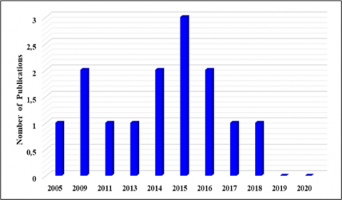
Unfortunately, there are fewer works mentioned in the literature related to the modelling of ANNs and the efficiency of NF/RO desalination plants (Figure 1).
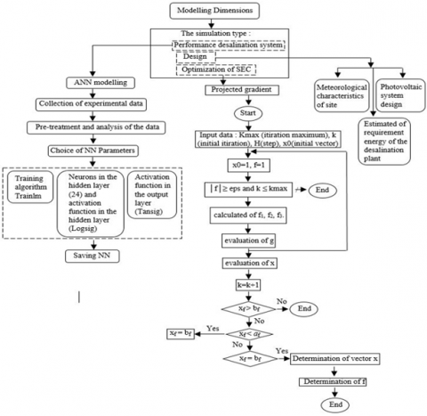
In the current work, the increasing needs for the water quality and energy consumption pushed us to investigate the potential of artificial neural network (ANN) model to estimate the efficiency of a NF/RO-PV seawater desalination system and to optimize the consumption energy of the system through the schema shown in Figure 2.
The schematic diagram of the main pillars of modelling dimensions was considered as an ideal structure for this work.
Figure 1. Number of published works on ‘NF/SWRO’ and ‘ANN’, from 1996 to 2020 [20]
Figure 2. Schematic diagram of NF/SWRO-PV modelling dimensions
2.1 Experimental data
The Saline Water Desalination Research Institute (SWRI) [21] provided the experimental NF/SWRO desalination plant data was utilized for building the ANN model. A pilot plant testing in which the nano-filtration membrane NF product is sent to the RO unit and its brine reject is utilized as a make-up for the MSF plant. The NF unit received pre-treated seawater with a temperature feed varying in 24 - 34℃ and was operated at a pressure about 23.54 bar and at a recovery of 53-57%.
In the SWRO unit receiving the NF product as feed, the pressure was fixed at 58.86 bar and the temperature varied in the range 23 – 34℃, where the average permeates recovery of the 1st and 2nd vessels were 30 and 21%, respectively. But, the overall recovery the SWRO system was about 45%.
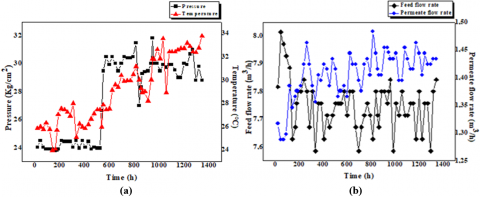
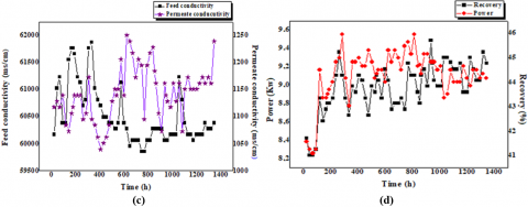
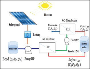
Figure 3 shows the diagram of the hybrid NF/RO desalination pilot system. The variation of the operating parameters of nanofiltration membrane (the pressure, temperature, conductivity, and the flow) as a function of time will be considered as inputs of the ANN model. However, the permeate conductivity, flow rate and recovery of the SWRO will be the outputs (Figure 4).
The values of the standard deviations (STD), mean (Mean), minimum (Min), and maximum (Max) of the used database are shown in Table 1.
Figure 3. Hybrid NF/RO seawater desalination pilot plant system [21]
Figure 4. Experimental data of performance parameters of hybrid system NF/RO
2.2 Neural network modelling
Artificial Neural Networks (ANNs) provides an appropriate control strategy for the controlled process [22, 23]. The feed forward neural network (FFNN) is one of the most used neural network paradigms in modelling a wide range of nonlinear systems, such as the biological and chemical engineering processes [24, 25]. It has been utilized here with forecasting horizon and supervised learning. The artificial neural network (ANN) algorithm is used to simulate the permeate flow rate and overall recovery (i.e., target variables). Sixty experiments were conducted for different values of the following parameters (Table 1): the time (h), temperature (℃), pressure (bar), feed conductivity, feed flow rate and power (kW).
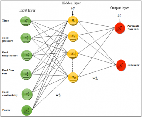
Figure 5 presents the schematic diagram of an artificial neural network (ANN) where six input neurons were set at the input layer. The permeate recovery, permeate conductivity, and permeate flow were determined for the two output neurons taken at the output layer.
A neural network with eight hidden layers selected experimentally has given satisfactory results for solving the present problem. While training data of very small size may prevent learning. Each node within a given layer is connected to all the nodes of the previous layer. A formal neuron is characterized by Eqns. (1) and (2):
$x_{i}=f\left(Z_{i}\right)$ (1)
$Z_{j}=f_{h}\left(\sum_{i=1}^{n} w_{j i}^{L} x_{i}+b_{h j}\right)$ (2)
j = 1, 2,.., m.
As highlighted by Eq. (3), the obtained value is propagated through outgoing connections to the neurons of the succeeding layer, where it undergoes the same process. For example, the outputs Zi of the hidden layer fed to neuron k of the output layer gives the output Sk:
$S_{k}=f_{0}\left(\sum_{i=1}^{m} w_{j k}^{h} z_{i}+b_{0 k}\right)$ (3)
k = 1, 2,.., l. l is the number of neurons in output layer.
Table 1. Description of the desalination pilot data
|
Variable category |
Parameters |
Symbol |
Unit |
STD |
Mean |
Min |
Max |
|
Inputs |
Time |
t |
h |
385.92 |
680.317 |
25.197 |
1343.830 |
|
pressure |
p |
Bar |
2.821 |
27.079 |
23.315 |
31.233 |
|
|
temperature |
T |
°C |
2.7422 |
29.063 |
23.968 |
33.789 |
|
|
Power |
P |
kW |
0.2661 |
8.992 |
8.239 |
9.487 |
|
|
Feed flow rate |
Jf |
m3/h |
0.088 |
7.748 |
7.586 |
8.014 |
|
|
Feed conductivity |
δf |
μS/cm |
535.010 |
60519.500 |
59851.060 |
61872.340 |
|
|
Outputs |
Permeate flow rate |
Jp |
m3/h |
0.042 |
1.406 |
1.288 |
1.483 |
|
Recovery |
y |
% |
1.018 |
44.308 |
41.093 |
45.951 |
Figure 5. Schematic diagram of an artificial neural network model
By combining Eqns. (3) and (2), the relation between the output Sk and the inputs xi of the ANN is obtained:
$S_{k}=f_{0}\left(\sum_{i=1}^{m} w_{j k}^{h} f_{h}\left(\sum_{i=1}^{n} w_{j i}^{l} x_{i}+b_{h j}\right)+b_{0 k}\right)$$ (4)
In this investigation, the log sigmoid (logsig) was utilized as transfer functions in the hidden layer (Eq. (5)) and the tangent sigmoid transfer function (Tansig) was used in the output layer (Eq. (6)). However, the (logsig) function, produces output in the range of -1 to +1 and the tansig transfer function produces outputs in the range of -∞ to +∞ [26].
$Z(x)=\frac{1}{1+e^{-x}}$ (5)
$Z(x)=\frac{e^{x}-e^{-x}}{e^{x}+e^{-x}}$ (6)
The normalization is needed if the ranges of the input data are different. All the training data were normalized in this research between -1 and 1, by using Eq. (7):
$x_{\text {norm}}=\frac{2\left(x_{i}-\min \left(x_{\mathrm{i}}\right)\right)}{\max \left(x_{i}\right)-\min \left(x_{i}\right)}-1$ (7)
here xi in the input or output variable x, xmax and xmin are equal to the maximum and minimum values noted for each variable of x. In order to determine the ANN system’s model, a program of the neural network is performed using Matlab (R2016b version).
2.3 Statistical analysis
The statistical parameters of the optimal NN model and performance prediction are the correlation coefficient R, the root mean square error RMSE (square root of the average sum of squares) and mean absolute error (MAE) [27] calculated for the predicted permeate flow rate and recovery. The equations are expressed as:
$R=\frac{\sum_{i}\left(y_{\text {exp}}-\overline{y_{\text {exp}}}\right)\left(y_{\text {cal}}-\overline{y_{\text {cal}}}\right)}{\sqrt{\sum_{i}\left(y_{\text {exp}}-\overline{y_{\text {exp}}}\right)^{2}} \sqrt{\sum_{i}\left(y_{\text {cal}}-\overline{y_{\text {cal}}}\right)^{2}}}$ (8)
$R M S E=\sqrt{\frac{1}{N} \sum_{i=1}^{N}\left(y^{e x p}-y^{c a l}\right)^{2}}$ (9)
$M A E=\frac{1}{N} \sum_{i=1}^{N}\left|\left(Y_{\text {exp}}-Y_{\text {cal}}\right)\right|$ (10)
Here N is the number of experiments, yexp is the experimental value for each parameter, ycal is the predicted value of the ith experiment calculate by the model for each parameter. $\bar{y}_{\exp }$ and $\bar{y}_{c a l}$ are the arithmetic mean of experimental and calculated values, respectively. Several techniques are available today, some of them may be used with minor modifications, while others are not suitable for this specific type of data set.
3.1 Model performance
The network was trained in this study using all 60 data points. The number of iterations for finding an adequate ANN model is 504 and the MSE is 2.9503×10⁻¹⁰.
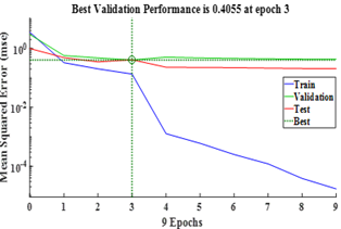
Figure 6. Diagram of MSE as function the number of iteration (epochs)
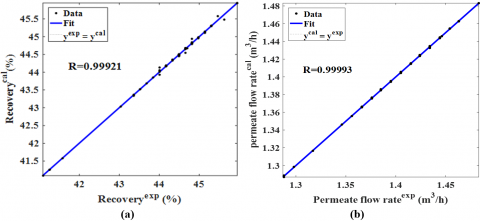
Figure 7. Experimental and predicted values from ANN model of (a) recovery and (b) permeate flow rate, respectively
Table 2. Linear regression vectors [linear equation]: $y^{\text {predict}}=a y^{\exp }+b, R, R M S E, M A E$.
|
|
Permeate Flow rate $\left(m^{3} / h\right)$ |
Recovery (%) |
|
a |
0.9999 |
1.0005 |
|
b |
1.7125 10-4 |
-0.0225 |
|
R |
0.9992 |
0.9999 |
|
RMSE |
0.0409 |
0.00048 |
|
MAE |
0.0213 |
3.7 10-4 |
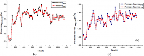
Figure 8. Simulation of experimental and predicted values of (a) recovery and (b) permeate flow rate, respectively
Figure 6 shows the performance of the trained ANN model where it is observed in first that the error decreases in few iterations (fast training) after it is stabilized until the convergence to the maximum number of epochs. The trained network was then simulated by feeding it with all of the data used for training. Figure 7 shows the predictive values of the network versus experimental values. An attempt is conducted to predict the recovery and permeate flow rate of the hybrid NF/RO process for seawater desalination treatment, aiming to enhance the water quality and reduce the production costs.
Through the analysis, Table 2 summarizes the model statistical parameters obtained by using the MATLAB function “postreg”, [a, b, R] = [1.0005, -0.0225, 0.9992] for the overall recovery; [a, b, R] = [0.999, -1.7125 10-4, 0.9999] for the permeate flow rate.
The results given by the ANN code are similar to the experimental data. The optimal structure corresponds to the correlation coefficient for NN 6-24-2 are 0.999935 and 0.99921, respectively for the permeate flow fate and overall recovery. A small means absolute error (MAE) and root mean square (RMSE) for the permeate flow fate and overall recovery.
The comparison between the experimental values and those calculated by ANN is presented in Figure 8, where an acceptable agreement is observed.
3.2 Mathematical equations of ANN developed model
The weights and bias of the optimized ANN models are given in Table 3, where WI is the input and hidden layer connection weight matrix, WH is the hidden and output layer connection weight matrix, bH is the hidden neurons bias and b° is the output neuron bias.
From the optimized ANN, we can express recovery (y) and permeate flow rate (Jp) by a mathematical model that incorporates all inputs xi (time, temperature, pressure, conductivity feed, flow rate feed and power is given by Eq. (11). Knowing that fh is the Logsig sigmoid transfer function used in hidden layer:
$Z_{j}=f_{h}\left[\sum_{i=1}^{6} w_{j i} x_{i}+b_{1}^{h}\right]$$=\frac{1}{1+\exp \left(-\sum_{i=1}^{6} w_{j i} x_{i}+b_{1}^{h}\right)}$ (11)
j = 1, 2, …, 24. The instance outputs Zj of the hidden layer are the output y and Jp (Eq. (12)). The combination of equations (12) and (13) leads to the mathematical formula for recovery and permeate flow rate taking into account all the inputs xi (Eq. (13)).
These mathematical formulas were used for the calculation of the recovery and permeate flow rate, and to predict the performance of the NF-SWRO hybrid seawater treatment. The prediction was achieved by including important relevant features that may be easily applied in controlling the desalination systems.
Combining the desalination with renewable energies is a way to reduce the energy consumption in seawater desalination processes [28]. The energy expenditure can exceed the half of the cost of operation for each process [29, 30]. The overall cost including the production of water and the energy consumption of these systems strongly depends on the specific parameters of each technology. The energy requirements of the NF-SWRO hybrid me
$y, J_{p}=f_{0}\left[\sum_{i=1}^{24} w_{j i}^{H} Z_{i}+b_{2}^{0}\right]=$$\frac{\exp \left(\sum_{i=1}^{24} w_{j i}^{H} Z_{i}+b_{2}^{0}\right)-\exp \left(-\Sigma_{i=1}^{24} w_{j i}^{H} Z_{i}+b_{2}^{0}\right)}{\exp \left(\sum_{i=1}^{24} w_{j i}^{H} Z_{i}+b_{2}^{0}\right)+\exp \left(-\Sigma_{i=1}^{24} w_{j i}^{H} Z_{i}+b_{2}^{0}\right)}$ (12)
$y, J_p=\frac{\exp \left(\sum_{i=1}^{24} w_{j i}^{H}\left(\frac{1}{1+\exp \left(-\sum_{i=1}^{6} w_{j i} x_{i}+b_{1}^{h}\right)}\right)+b_{2}^{0}\right)-\exp \left(-\sum_{i=1}^{24} w_{j i}^{H}\left(\frac{1}{1+\exp \left(-\sum_{i=1}^{6} w_{j i} x_{i}+b_{1}^{h}\right)}\right)+b_{2}^{0}\right)}{\exp \left(\sum_{i=1}^{24} w_{j i}^{H}\left(\frac{1}{1+\exp \left(-\sum_{i=1}^{6} w_{j i} x_{i}+b_{1}^{h}\right)}\right)+b_{2}^{0}\right)+$\exp \left(-\sum_{i=1}^{24} w_{j i}^{H}\left(\frac{1}{1+\exp \left(-\sum_{i=1}^{6} w_{j i} x_{i}+b_{1}^{h}\right)}\right)+b_{2}^{0}\right)}$(13)
Table 3. Weights and bias of the optimized NN model
|
Input and hidden layer connections |
Hidden layer and output connections |
||||||||
|
$\boldsymbol{W}^{I}$ |
$\boldsymbol{b}_{1}^{H}$ |
$W^{H}$ |
$\boldsymbol{b}_{2}^{0}$ |
||||||
|
$t(h)$ |
$P($bar$)$ |
$T\left({ }^{\circ} C\right)$ |
$J_{f}\left(m^{3} / h\right)$ |
$\delta_{f}(\mu s / c m)$ |
$P(k W)$ |
$y$ |
$J_{p}\left(m^{3} / h\right)$ |
||
|
-0.00022 |
-0.00049 |
-0.24238 |
-0.24452 |
-0.18530 |
0.00134 |
3.18595 |
-0.00493 |
4.93906 |
|
|
-0.00013 |
0.00007 |
-0.43411 |
1.49330 |
-0.44865 |
-0.00066 |
-2.99437 |
-0.00130 |
4.11969 |
|
|
0.00002 |
0.00029 |
1.16235 |
1.64378 |
-0.25506 |
-0.00104 |
-0.60247 |
0.00008 |
-0.00312 |
|
|
0.00034 |
-0.00005 |
2.55987 |
0.20847 |
0.23936 |
-0.00107 |
-0.54756 |
0.00391 |
-0.00037 |
|
|
0.00016 |
0.00033 |
-1.03864 |
1.37116 |
0.22075 |
0.00010 |
1.18852 |
4.83447 |
-3.43846 |
|
|
0.00009 |
0.00053 |
2.91488 |
1.89925 |
-0.99727 |
-0.00086 |
1.87594 |
-0.00513 |
-0.00680 |
|
|
1.98547 |
-0.00046 |
-0.69812 |
0.00063 |
-1.15051 |
0.00323 |
-1.44032 |
-3.57866 |
0.00834 |
|
|
2.33267 |
-0.00026 |
-0.10148 |
0.00179 |
0.01060 |
-0.00093 |
0.63800 |
0.22776 |
-4.93655 |
|
|
1.54040 |
-0.00003 |
1.19866 |
0.00085 |
2.13683 |
-0.00169 |
-1.87212 |
-0.42809 |
4.16520 |
|
|
-0.77783 |
0.00037 |
1.60591 |
-0.00297 |
0.14919 |
-0.00089 |
-1.43780 |
-0.00063 |
0.17560 |
|
|
0.70447 |
0.00021 |
-0.23998 |
-0.00009 |
2.20851 |
-0.00033 |
2.04408 |
0.00291 |
0.00278 |
|
|
-0.50803 |
-0.00001 |
-0.52796 |
0.00438 |
-2.66601 |
-0.00298 |
-0.37095 |
-5.33116 |
5.37838 |
|
|
0.00181 |
0.00150 |
-0.00034 |
0.01512 |
-0.00001 |
-2.84990 |
-2.79447 |
0.00262 |
0.05018 |
-1.92521 |
|
-0.00124 |
-0.00011 |
-0.00001 |
-0.06365 |
-0.00095 |
-0.82540 |
-0.27675 |
-0.00823 |
-0.04616 |
1.88754 |
|
-0.00094 |
-0.00013 |
0.00018 |
0.41999 |
-0.00018 |
-0.98313 |
-4.56674 |
0.00171 |
0.00062 |
|
|
0.00020 |
-0.00150 |
0.00038 |
-0.24045 |
0.00026 |
0.72625 |
-5.17365 |
-0.00397 |
-0.00377 |
|
|
-0.00022 |
0.00000 |
-0.00013 |
-0.06758 |
0.00015 |
0.59016 |
-0.84911 |
-0.02195 |
-0.33057 |
|
|
-0.00291 |
-0.00013 |
0.00012 |
3.53384 |
-0.00127 |
-0.64655 |
1.34461 |
0.00150 |
-0.01339 |
|
|
1.91034 |
0.00049 |
0.00181 |
6.22952 |
0.38450 |
-0.82229 |
-2.00470 |
-0.05718 |
0.00758 |
|
|
-0.83535 |
-0.00061 |
-0.00120 |
1.37660 |
0.32993 |
-1.05713 |
1.25119 |
4.12923 |
0.04144 |
|
|
-1.76895 |
-0.00051 |
-0.00064 |
1.05375 |
0.09944 |
0.88303 |
0.16639 |
-1.59597 |
-0.10482 |
|
|
0.91538 |
0.00021 |
0.00192 |
-2.52199 |
-0.41873 |
-2.88922 |
0.07895 |
-0.00673 |
-1.70748 |
|
|
1.72058 |
-0.00006 |
-0.00083 |
0.93180 |
-0.20638 |
-1.59650 |
4.59911 |
-0.00325 |
-0.01000 |
|
|
0.18731 |
-0.00145 |
-0.00564 |
-0.42074 |
-0.91719 |
1.12731 |
0.04285 |
0.17993 |
-0.19405 |
|
4.1 Dimensioning of the photovoltaic system for a desalination plant
The photovoltaic systems are used today in small-scale desalination plants. The photovoltaic is needed for the system power input. The PV module is expected to operate directly with the NF/SWRO during eight hours per day (Figure 9). The elements of the PV system are: a PV module, an electric inverter unit (convert DC to AC), a distribution cabinet, cables, and an array power 150 Watt/array with 24V.
Figure 9. NF/RO/PV seawater desalination pilot plant system
4.1.1 Meteorological data and location of the operation
A seawater desalination pilot without an energy recovery system installed in Saudi Arabia was composed of NF membrane for pre-treatment and RO in post-treatment. The plant location is suitable to inspect the model. The average ambient temperature is around 11-35℃ along the year and a maximum of solar irradiation is recorded in June with a value close to 7 kWh/m2/day and a min in December. The meteorological operating conditions of the plant location are provided in Figure 10 [31].
Figure 10. Monthly average of solar radiation [31]
4.1.2 Estimated energy requirement of the desalination plant
The values of NF and SWRO operating parameters utilized in the operation of the dual NF-SWRO unit are given in Table 4.
Table 4. NF/SWRO unit parameters
|
Parameters |
NF/SWRO |
|
Recovery |
45% |
|
Feed pressure (bar) |
58.89 |
|
Feed flow rate (m3/h) |
8.014 |
|
Permeate flow rate (m3/h) |
1.406 |
The energy requirements during the seawater desalination by NF-SWRO membrane processes were calculated for the part desalination only from the general equation [32]:
$S E C=\frac{Q_{f} * H_{f} * g}{366 * Q_{P} * e}$ (14)
The specific energy consumption equation of the NF-SWRO process is presented as:
$S E C_{\text {des},(N F-S W R O)}=$$\frac{\left(Q_{f_{(N F)}} * H_{f_{(N F)}} * g\right)+\left(Q_{f_{(S W R O)}} * H_{f_{(S W R O)}} * g\right)}{\left(366 * Q_{P_{(F i n a l)}} * e\right)}$ (15)
where, the sec in kWh/m3, Qf and Qp are the feed and permeate flow rate (m3/h), respectively. Hf is the pressure head (m), g is the specific gravity of seawater (1.03), and e is the pump efficiency (≈0.85). The SEC of the dual NF-SWRO, process was calculated from Eq. (17) and the power of the plant is calculated for a pumping time per day (5 hours) as follow:
$P_{D E S}=\sec \times Q_{p} \times 5 h / d a y$ (16)
4.1.3 Modelling of the PV modules
The energy consumption of the desalination unit, which is determined based on the values of the flow rate and feed pressure, is used to model the photovoltaic PV. In this configuration, the PV system is connected to a battery unit to drive the NF-SWRO desalination unit.
Battery Storage:
In this configuration, PV is coupled to batteries whose state of charge and discharge control the operation of the desalting system. The nominal capacity calculation of the battery takes into account the needs and the days of autonomy, as well as the depth of discharge. The batteries capacity is determined as:
$\mathrm{C}=\frac{\mathrm{N}_{\mathrm{a}} \mathrm{E}_{\mathrm{C}}}{\mathrm{UP}_{\mathrm{d}}}$ (17)
where, Pd is the discharge depth (0.7 to 0.8), EG is the consumption energy, U is the DC system voltage (volt), and Na is the battery autonomy days (5 days).
A suitable charge regulator was used in the PV-NF/SWRO system with the specification of 12 V/24 V.
PV panels:
The power generated by the PV system is expressed as [33]:
$P p v_{\text {, } \bmod }=0.001 \times P_{\text {pv,tot}} \times t_{h d}$ (18)
$P_{P V, t o t}=\frac{P_{D E S}}{t_{h d} / 24+\left(1-t_{h d} / 24\right) \alpha_{B C H} \alpha_{B D C H}}$ (19)
where, Ppv,arr is the module photovoltaic power (kW/h/m2/day), Ppv,tot is the power energy of photovoltaic system, thd is the hourly solar insolation (about 7 h/j). αBCH and αBDCH αBDCH are the battery efficiency charge and discharge, respectively. The number of modules necessary to power the NF-SWRO unit is calculated for a module of 150 Wc capacity by the following equation [33]:
$N_{\text {mod}}=\frac{1}{t_{h d} / 24+\left(1-t_{h d} / 24\right) \alpha_{B C H} \alpha_{B D C H}} \frac{P_{D E S}}{P_{\text {PVarr}}}$ (20)
Following the design method, Table 5 presents the performance parameters of the photovoltaic system desalination plant.
Table 5. Summary of design NF/RO/PV system parameters
|
Parameters |
Values |
|
|
NF/RO unit |
SEC |
6.397 kWh/m3 |
|
Pdes |
44.97 kWh |
|
|
PV system |
Cbatt |
58.32 kWh |
|
Ppv,tot |
111.98 kWh/day |
|
|
Ppv,mod |
0.77 kWh/day |
|
|
Nmod |
148 modules |
4.2 Optimization of the specific energy consumption
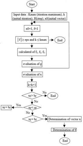
A program on Matlab has been established to minimize the specific consumption energy of desalination plant, based on the projected gradient decent (PGD) method under constraint algorithms (Figure 11).
The principle of the method is based on the gradient calculation of the objective function based on various parameters and recalculates, under constraints in order to assess the specific energy consumption. The PGD method is based on the usual gradient methods.
Supposing that we want to solve the constrained optimization problem, where $f$ is a convex function [34] . $\min f\left(x_{j}\right)_{x \in R^{n}} ;$ If we wish to use gradient descent update to a point $x_{t} \in R,$ it is possible that the iterate $x_{t+1}=x_{t}-\alpha \nabla f\left(x_{t}\right)$ may not belong to the constraint setR. In the projected gradient descent, we simply choose the point nearest to $x_{t}-\alpha \nabla f\left(x_{t}\right)$ in the set $R$ as $x_{t+1}$.
Given a starting point $x_{0} \in R$ and step-size $\left.\gamma\right\rangle 0,$ PGD works as follows until a certain stopping criterion is satisfied:
$\left\|x_{t+1}-x_{t}\right\|>\varepsilon, \varepsilon>0$ (21)
In this configuration, the unit of desalination is without a recovery system. However, the high-pressure pump is considered as a recovery system. The energy required to produce 1.406 m3/h is of the order of 6.397 kWh/m3. According to the literature, the specific energy for the production of one cubic meter of treated water without energy recovery is between 6 and 7.5 kWh/m3. This value depends on the Physico-chemical characteristics of seawater.
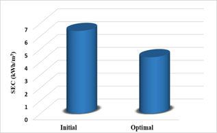
The program recalculates the values and gives the optimum values of the operational parameters. The initial value of the specific energy consumption (SEC) is of the order 6.397 kWh/m3 after the execution of the program. The optimal value is 4.36 kWh/m3 with an error of 31.8% (Figure 12).
Finally, the performance of the electricity cell may be improved based on the heat exchangers [35-46] in order to reduce its temperature and increase its efficiency as a future study.
Figure 11. Flowchart of projected method
Figure 12. Results of the program using the projected gradient method
Aiming to control the operation of a hybrid NF/RO seawater desalination unit, a feed-forward artificial neural network was used for the development of a model able to predict the permeate flow rate and recovery. The analyses of the results showed that the ANN models were good for the prediction of flow rate and recovery with high R2, and low RMSE and MAE values.
An ANN model used as control system tools for a small-scale prototype NF/SWRO desalination plant was tested. The design and sizing of the PV-NF/SWRO unit components was presented.
The energy needs of seawater desalination are such that they constitute the largest share of operating desalination costs. In this paper, an optimization of the specific consumption energy (SEC) of the unit was achieved. The projected gradient method under MATLAB Environment software was utilized to solve the corresponding equation. The program minimized the SEC of the desalination unit up to 38%.
The authors gratefully acknowledge the Algerian Ministry of Higher Education and Scientific Research and Laboratory of Biomaterials and Transport Phenomena (LBMPT) of University Yahia Fares of Medea, Algeria.
[1] Ellabban, O., Abu-Rub, H., Blaabjerg, F. (2014). Renewable energy resources: Current status, future prospects and their enabling technology. Renewable and Sustainable Energy Reviews, 39: 748-764. https://doi.org/10.1016/j.rser.2014.07.113
[2] Sabry, M., Nahas, M., AlLehyani, S. (2015). Simulation of standalone portable steam generator driven by a solar centrator. Energies, 8(5): 3867-3881. https://doi.org/10.3390/en8053867
[3] Pérez-González, A., Ibáñez, R., Gómez, P., Urtiaga, A.M., Ortiz, I., Irabien, J.A. (2015). Nanofiltration separation of polyvalent and monovalent anions in desalination brines. J. Membrane Science, 473: 16-27. https://doi.org/10.1016/j.memsci.2014.08.045
[4] Rodríguez-Calvo, A., Silva-Castro, G.A., Osorio, F., López, J.G., Calvo, C. (2015). Reverse osmosis seawater desalination: Current status of membrane systems. Desalination and Water Treatment, 56(4): 849-861. https://doi.org/10.1080/19443994.2014.942378
[5] Fritzmann, C., Löwenberg, J., Wintgens, T., Melin, T. (2007). State-of-the-art of reverse osmosis desalination. Desalination, 216(1-3): 1-76. https://doi.org/10.1016/j.desal.2006.12.009
[6] Kaya, C., Jarma, Y.A., Guler, E., Kabay, N., Arda, M., Yükse, M. (2020). Seawater desalination by using nanofiltration (NF) and Brackish Water Reverse Osmosis (BWRO) membranes in sequential mode of operation. Journal of Membrane Science Research, 6(1): 40-46. http://dx.doi.org/10.22079/JMSR.2019.107844.1264
[7] Diawara, K.C. (2008). Nanofiltration process efficiency in water desalination. Separation & Purification Reviews, 37(3): 302-324. https://doi.org/10.1080/15422110802228770
[8] Hilal, N., Al-Zoubi, H., Darwish, N.A., Mohamma Arabi, M.A. (2004). A comprehensive review of nanofiltration membranes: Treatment, pretreatment, modelling, and atomic force microscopy. Desalination, 170(3): 281-308. https://doi.org/10.1016/j.desal.2004.01.007
[9] Khawaji, A.D., Kutubkhanah, I.K., Wie, J.M. (2008). Advances in seawater desalination technologies. Desalination, 221(1-3): 47-69. https://doi.org/10.1016/j.desal.2007.01.067
[10] AlTaee, A., Sharif, A.O. (2011). Alternative design to dual stage NF seawater desalination using high rejection brackish water membranes. Desalination, 273(2-3): 391-397. https://doi.org/10.1016/j.desal.2011.01.056
[11] Ghermandi, A., Messalem, R. (2009). Solar-driven desalination with reverse osmosis: the state of the art. Desalination and Water Treatment., 7(1-3): 285-296. https://doi.org/10.5004/dwt.2009.723
[12] Ben Meriem, A., Bouguecha, S., ElsayedAly, S. (2013). Solar-driven integrated RO/NF for water desalination. International Journal of Engineering Research and Applications, 3(1): 354-368.
[13] Shen, J., Mkongo, G., Abbt-Braun, G., Ceppi, S.L., Richards, B.S., Schäfer, A.I. (2015). Renewable energy powered membrane technology: fluoride removal in a rural community in northern Tanzania. Separation and Purification Technology, 149: 349-361. https://doi.org/10.1016/j.seppur.2015.05.027
[14] Suykens, J.A., Vandewalle, J.P., De Moor, B.L.R. (1996). Artificial Neural Networks for Modelling and Control of Non-Linear Systems. Springer, 1st edition (1996). http://dx.doi.org/10.1007/978-1-4757-2493-6
[15] El-Hawary, M.E. (1993). Artificial neural networks and possible applications to desalination. Desalination. 92(1-3): 125-147. https://doi.org/10.1016/0011-9164(93)80078-2
[16] Murthy, Z.V.P., Vora, M.M. (2004). Prediction of reverse osmosis performance using artificial neural network. Indian Journal of Chemical Technology, 11(1): 108-115.
[17] Abbas, A., Al-Bastaki, N. (2005). Modeling of an RO water desalination unit using neural networks. Chemical Engineering Journal, 114(1-3): 139-143. https://doi.org/10.1016/j.cej.2005.07.016
[18] Gao, P., Zhang, L., Cheng, K., Zhang, H. (2007). A new approach to performance analysis of a seawater desalination system by an artificial neural network. Desalination, 205(1-3): 147-155. https://doi.org/10.1016/j.desal.2006.03.549
[19] Aish, A.M., Zaqoot, H.A., Abdeljawad, S.M. (2015). Artificial neural network approach for predicting reverse osmosis desalination plants performance in the Gaza Strip. Desalination, 367: 240-247. https://doi.org/10.1016/j.desal.2015.04.008
[20] www.scienceDirect.com, accessed on 11/06/2020.
[21] Hamed, O.A., Hassan, A.M., Al-Shail, K., Farooque, M.A. (2009). Performance analysis of a trihybrid NF/RO/MSF desalination plant. Desalination and Water Treatment, 1(1-3): 215-222. https://doi.org/10.5004/dwt.2009.113
[22] Ammi, Y., Khaouane, L., Hanini, S. (2015). Prediction of the rejection of organic compounds (neutral and ionic) by nanofiltration and reverse osmosis membranes using neural networks. Korean Journal of Chemical Engineering, 32(11): 2300-2310. https://doi.org/10.1007/s11814-015-0086-y
[23] Maouz, H., Khaouane, L., Hanini, S., Ammi, Y. (2019). Modeling the molecular weight and number average molecular masses during the photo-thermal oxidation of polypropylene using neural networks. Moroccan Journal of Chemistry, 7(1): 017-027.
[24] Siham, C.M., Salah, H., Maamar, L., Latifa, K. (2017). Artificial neural networks based prediction of hourly horizontal solar radiation data: Case study. International Journal of Applied Decision Sciences, 10(2): 156. https://doi.org/10.1504/ijads.2017.084312
[25] Hamadache, M., Benkortbi, O., Hanini, S., Amrane, A., Khaouane, L., Moussa, C.S. (2016). A quantitative structure activity relationship for acute oral toxicity of pesticides on rats: Validation, domain of application and prediction. Journal of Hazardous Materials, 303: 28-40. https://doi.org/10.1016/j.jhazmat.2015.09.021
[26] Adda, A., Hanini, S., Abbas, M., Sediri, M. (2019). Novel adsorption model of filtration process in polycarbonate track-etched membrane: Comparative study. Environmental Engineering Research, 25(4): 479-487. https://doi.org/10.4491/eer.2019.136
[27] Hamadache, M., Hanini, S., Benkortbi, O., Amrane, A., Khaouane, L., Moussa, C.S. (2016). Artificial neural network-based equation to predict the toxicity of herbicides on rats. Chemometrics and Intelligent Laboratory Systems, 154: 7-15. https://doi.org/10.1016/j.chemolab.2016.03.007
[28] Viola, A., Franzitta, V., Trapanese, M., Curto, D., Viola, D. (2016). Nexus water & energy: A case study of wave energy converters (WECs) to desalination applications in Sicily. International Journal of Heat and Technology, 34(S2): S379-S386. https://doi.org/10.18280/ijht.34S227
[29] Goosen, M., Mahmoudi, H., Ghaffour, N. (2010). Water desalination using geothermal energy. Energies, 3(8): 1423-1442. https://doi.org/10.3390/en3081423
[30] Ghaffour, N. (2009). The challenge of capacity-building strategies and perspectives for desalination for sustainable water use in MENA. Desalination and Water Treatment, 5(1-3): 48-53. https://doi.org/10.5004/dwt.2009.564
[31] Rehman, S., Ahmed, M.A., Mohamed, M.H., Al-Sulaiman, F.A. (2017). Feasibility study of the grid connected 10 MW installed capacity PV power plants in Saudi Arabia. Renewable and Sustainable Energy Reviews, 80: 319-329. https://doi.org/10.1016/j.rser.2017.05.218
[32] Ahunbay, M.G., Tantekin-Ersolmaz, S.B., Krantz, W.B. (2018). Energy optimization of a multistage reverse osmosis process for seawater desalination. Desalination, 429: 1-11. https://doi.org/10.1016/j.desal.2017.11.042
[33] Filippini, G., Al-Obaidi, M.A., Manenti, F., Mujtaba, I.M. (2019). Design and economic evaluation of solar-powered hybrid multi effect and reverse osmosis system for seawater desalination. Desalination, 465: 114-125. https://doi.org/10.1016/j.desal.2019.04.016
[34] Nesterov, Y. (2004). Introductory Lectures on Convex Optimization: A Basic Course. Springer US. https://doi.org/10.1007/978-1-4419-8853-9
[35] Menni, Y., Chamkha, A.J., Zidani, C., Benyoucef, B. (2020). Analysis of thermo-hydraulic performance of a solar air heater tube with modern obstacles. Archives of Thermodynamics, 41(3): 33-56. https://doi.org/10.24425/ather.2020.134571
[36] Chamkha, A.J., Menni, Y. (2020). Hydrogen flow over a detached v-shaped rib in a rectangular channel. Mathematical Modelling of Engineering Problems, 7(2): 178-186. https://doi.org/10.18280/mmep.070202
[37] Menni, Y., Chamkha, A.J., Makinde, O.D. (2020). Turbulent heat transfer characteristics of a W-baffled channel flow - heat transfer aspect. Defect and Diffusion Forum, 401: 117-130. https://doi.org/10.4028/www.scientific.net/DDF.401.117
[38] Menni, Y., Chamkha, A.J., Azzi, A., Zidani, C. (2020). Numerical analysis of fluid flow and heat transfer characteristics of new kind of vortex generators by comparison with those of traditional vortex generators. International Journal of Fluid Mechanics Research, 47(1): 23-42. https://doi.org/10.1615/InterJFluidMechRes.2019026753
[39] Menni, Y., Azzi, A., Chamkha, A. (2019). Computational thermal analysis of turbulent forced convection flow in an air channel with a flat rectangular fin and downstream V-baffle. Heat Transfer Research, 50(18): 1781-1818. https://doi.org/10.1615/HeatTransRes.2019026143
[40] Sakhri, N., Draoui, B., Menni, Y. (2019). Experimental study of earth to air heat exchanger performance in arid region. First step: in - situ measurement of ground vertical temperature profile for different depths. Journal of Advanced Research in Fluid Mechanics and Thermal Sciences, 56(2): 183-194.
[41] Menni, Y., Chamkha, A.J., Zidani, C., Benyoucef, B. (2019). Numerical analysis of heat and nanofluid mass transfer in a channel with detached and attached baffle plates. Mathematical Modelling of Engineering Problems, 6(1): 52-60. https://doi.org/10.18280/mmep.060107
[42] Menni, Y., Chamkha, A.J., Zidani, C., Benyoucef, B. (2019). Heat and nanofluid transfer through baffled channels in different outlet models. Mathematical Modelling of Engineering Problems, 6(1): 21-28. https://doi.org/10.18280/mmep.060103
[43] Menni, Y., Chamkha, A.J., Zidani, C., Benyoucef, B. (2019). Heat transfer in air flow past a bottom channel wall-attached diamond-shaped baffle - using a CFD technique. Periodica Polytechnica Mechanical Engineering, 63(2): 100-112. https://doi.org/10.3311/PPme.12490
[44] Menni, Y., Azzi, A., Chamkha, A.J. (2019). Modeling and analysis of solar air channels with attachments of different shapes. International Journal of Numerical Methods for Heat & Fluid Flow, 29(5): 1815-1845. https://doi.org/10.1108/HFF-08-2018-0435
[45] Menni, Y., Azzi, A., Chamkha, A.J. (2019). The solar air channels: Comparative analysis, introduction of arc-shaped fins to improve the thermal transfer. Journal of Applied and Computational Mechanics, 5(4): 616-626. https://doi.org/10.22055/JACM.2018.26785.1356
[46] Menni, Y., Azzi, A., Chamkha, A.J. (2018). Turbulent heat transfer and fluid flow over complex geometry fins. Deflect and Diffusion Forum, 388: 378-393. https://doi.org/10.4028/www.scientific.net/DDF.388.378