Yanán Camaraza-Medina* | Andres A. Sánchez-Escalona | Yoalbys Retirado-Mediaceja | Osvaldo F. García-Morales
© 2020 IIETA. This article is published by IIETA and is licensed under the CC BY 4.0 license (http://creativecommons.org/licenses/by/4.0/).
OPEN ACCESS
In this paper is presented a new procedure for the calculation of the heat transfer in vertical and inclines tubes, with presence of viscous-gravitational flow. Three models, one for inclines tubes and two for vertical tubes with presence of downward and upward flow were developed. The first model was development for coincident directions and 12 different fluids, included water and organic liquids, shows a correlation adjustment with a mean error of 12.75% in 81.51 % of the available experimental data in the interval of validity $7.5 \times 10^{5} \leq \operatorname{Ra}<2.75 \times 10^{11}$ and $0.9<\operatorname{Pr} \leq 3.5 \times 10^{4}$. The second model was development for not coincident directions and 10 different fluids, included water and organic liquids, shows a correlation adjustment with a mean error of 13.04% in 83.09 % of the available experimental data in the interval of validity $7.6 \times 10^{5} \leq \mathrm{Ra}<1.45 \times 10^{11}$ and $0.8<\operatorname{Pr} \leq 3.9 \times 10^{4}$. The third model was development for inclined tubes, it is valid for 10 different fluids included water and organic liquids, shows a correlation adjustment with a mean error of 16.12%, in 81.08% of the available experimental data in the interval of validity $7.9 \times 10^{5} \leq \mathrm{Ra}<6.98 \times 10^{10}, 0.9<\operatorname{Pr} \leq 2.1 \times 10^{4}$ and angle of inclination with respect to horizontal line $1^{\circ} \leq \theta \leq 88^{\circ}$. The objective of this paper is to make a procedure of analysis that enables considering the influence of the gravitational effects in the laminar flow regimen and to decrease the average uncertainty of the models and that additionally has a larger range of applicability.
rayleigh number, heat transfer coefficient, mean deviation, viscous-gravitational
In the thermal engineering, the evaluation of the heat transfer processes inside of tubes, two models of not isothermic laminar flow are possible: viscous and viscous-gravitational. Each one of them has their own laws of heat transfer.
In laminar flow, when it comes true than $R a \geq 8 \times 10^{5}$, then, the gravitational forces have influence of important way in the heat transfer, generating that the effect of the free convection cannot be rejected, therefore, the methods of analysis known for laminar flow does not allow obtaining satisfactory results. This type of problems is known as regimen of viscous-gravitational flow [1].
The viscous flow not isothermic appear when the forces of viscosity prevail over the gravitational forces, therefore, the viscous fluids do not receive the influence of the free convection. The viscous-gravitational flow appears when the gravitational forces are appreciable, and therefore, the natural convection adds to the forced. The model of viscous flow is so much more probable than the gravitational one, as much as the minor is the diameter of the tube, bigger the viscosity of the fluid and minor the temperature difference.
The velocity distribution in the cross section of the tube with viscous flow is not parabolic, due to the change of the viscosity with the temperature in the straightaway section. The velocity distribution is dependent if the fluid be heated or cooled (see Figure 1) [2].
Figure 1. Transverse circulation in a tube due to the free convection (heating and cooling)
For a same mean temperature in the cross section, the temperature for the fluid near of the wall is major when he gets heat, that when he gets cold. While the temperature of a liquid increases, viscosity decreases, therefore, the velocity of the fluid near of the tube wall, in the case of heating, is greater than in that of cooling, and therefore, velocity increases in the heat transfer [3, 4].
When the liquid heats, the superficial transmission factor of heat is major that when he gets cold, the difference between the coefficients is major as much as the difference of temperature is bigger. When the liquid is heat, the superficial transmission factor of heat is major that when he gets cold; The difference between the heat transfer coefficients is major as much as bigger is the temperature difference [5].
In addition to the effect of the viscosity variations, in a gravitational viscous flow the distribution of velocity is very influenced for intensity and the direction of the free convection, that originates as a consequence of the difference of densities between the hot and cold zones of the fluid [6, 7].
Therefore, the presence of the gravitational forces in the laminar flow regimen, makes complex the solution of the problem and reduces the precise grade in the obtained results, because the existing methods in literature do not consider this influence. Several investigators accomplished efforts to solve this inconvenience, however, the methods proposed only comprise reduced zones and close errors to the 30% [3].
Therefore, the authors follow as objective in this paper, developing a procedure of analysis that it enables considering the influence of the gravitational effects in the laminar flow regimen, that reduces the average level of uncertainty of the model and that additionally has a larger range of applicability.
2.1 Introductory elements on the gravitational viscous flow
In the practical engineering, three basic cases of viscous gravitational regimen can be found, which depend on the direction of the forced and free convection [3]:
Case 1: The natural and the forced convection have the same direction.
Case 2: The natural and the forced convection have perpendicular directions.
Case 3: The natural and the forced convection have opposed directions.
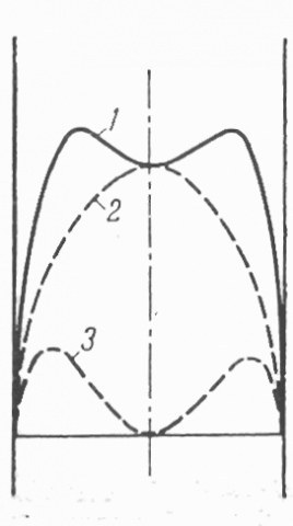
Case 1 is found in vertical tubes, when a fluid that move along the tube in upward direction while receive heat, or a fluid that circulates in downward direction and its cooling. In this case, the effect of the free convection produces an increase of the fluid velocity near of the wall (see Figure 2) and there can be two maximums in the diagram of velocities distribution [8, 9].
In Figure 2 below, the enumerated curves are:
Figure 2. Distribution of velocities in the cross section of a tube with forced and free convection in the same direction
Figure 3. Distribution of velocities in the cross section of a tube with forced and free convection in the contrary direction
Case 2 is found in horizontal pipes. Due to the free convection, in the normal section of the tube a cross-sectional circulation comes from the fluid. In a heated fluid appear currents of free convection, upwards for the side of the wall and downwards for the center of the tube, while in the case of fluid cooling, the opposite happens. In consequence, the fluid moves through the tube following a spiral. The velocity of heat transfer increases due to the improvement in the fluid mixed [10, 11].
Case 3 is found in vertical tubes, when a fluid that move along the tube in downward direction while receive heat, or a fluid that circulates in upward direction and its cooling. In this case, decrease the velocity of the fluid near the wall, because convection currents have opposed directions (see Figure 3), which generates the formation of vortexes in the fluid close to the wall. Therefore, the process intensifies and the heat transfer turns out to be bigger than in the two previous cases, due to the intermittent appearing of turbulent motion [12, 13].
At the present time, in the specialized literature, the existing methods do not cover up with enough exactness, the estimation of the heat transfer in viscous-gravitational regimen in inclined tubes. A criterion that enjoys certain popularity is Cebeci's method, however, his use looks limited to inclined tubes 30o with respect to horizontal line, for what flows water in downward direction [4, 5].
In Figure 3 above, the enumerated curves are:
By means of the dimensional analysis techniques, it is very easy to prove that the viscous –gravitational flow regimen is strongly influenced by Prandtl and Grashoff dimensionless numbers, the inner diameter of the tube and its length [14].
The investigations realized in the years 50 of the last century focused on the solution of this problem, however, in spite of the great quantity of experimental data generated, the obtained solutions are based on systems of the mathematical form Nu=aRemPrn, for what it was required to limit the expressions obtained to intervals reduced of applicability [15].
However, the viscous–gravitational flow regimen in horizontal pipes is largely studied; existing in the literature an important group of current contributions, for such motive is excluded of the interests and reaches of this paper.
For the analysis of the cases 1 and 3, in literature exist two procedures, however these show high errors of correlation and have reduced ranges of applicability. These methods come given for [16-18]:
For the case 1
$N u=0.35 G z^{0.3}\left[ R a \frac{d}{l}\right]^{0.18}$ (1)
Eq. (1) is valid for the following range of values:
$20<l / d \leq 130 ; \quad R e \leq 7.26 R a^{0.4}$
$8 \times 10^{5} \leq R a \leq 4 \times 10^{8} \quad ; \quad 1.5\left(R a \frac{d}{l}\right)^{0.25} \leq G z \leq 110$
Eq. (1) correlates with a 50% of average error.
For the case 3
$N u=0.037 R e^{0.75} \operatorname{Pr}^{0.4}\left(\mu_{F} / \mu_{P}\right)^{N}$ (2)
In Eq. (2), the constant N take values 0.11 and 0.25 for heating and cooling of the fluid respectively.
Eq. (2) is valid for the following range of values:
$0.2<\operatorname{Pr} \leq 100 ; 250<\operatorname{Re} \leq 10^{4}$
$1.5 \times 10^{6}<\operatorname{Re} \leq 12 \times 10^{6}$
The Eq. (2) correlates with a 40% of average error.
3.1 Deduction and validation of the proposal models
In the present paper, the experimental available data were obtained from an extended revision [3] compiled from literature specialized on the matter in Russian language [6-15], in which, were compiled and detailed an important group of experimental measurements on viscous gravitational flow, accomplished for investigators of the ancient Soviet Union. These experimental data will be used to achieve the adjustment and validation of the proposed models [19-21]. The study executed for the cases 1 and 3, as well as for inclined pipes, is given at once.
Case 1
Table 1 provides a summary of the experimental data used in the adjustment and validation of the proposal model for heat transfer calculation in viscous-gravitational flow for the case 1 [3]. The adjustment of the experimental available data is possible to realize it by means of a function of superposition (Brezhnetzov's function), establishing as fixed parameter the function Gr0.2 and as residue x0.48, in this case the residue is contingent upon the Prandtl number, in order to be the second experimental parameter in importance. The obtained model is given by:
$N u_{V 1}=\frac{0.69 P r^{0.48} G r^{0.2}(l / d)^{0.01}}{\left(0.61+1.2(P r+1.24 P r)^{0.48}\right)^{0.3}}+A$ (3)
In Eq. (3), if $\operatorname{Pr} \leq 10,$ then $A=0 .$ For $\operatorname{Pr}>10$ then this should be corrected by means of the addition of a constant, whose value can be obtained in the Table 2.
Table 3 is given the validity intervals of the Equation (3). The Table 4 shows the correlation index of the Equation (3) in eight sub-intervals of their validity range, being proved that the Eq. (3) provides a correlation adjustment with an average error of 12.75% in 81.51% of the experimental available data. Figure 4 represents the adjustment obtained (with a 15% error band) between Eq. (3) and the experimental data.
Case 3
Table 5 provides a summary of experimental data used in the adjustment and validation of the proposal model for heat transfer calculation in viscous-gravitational flow for case 3.
The adjustment of the experimental available allow to get that the heat transfer in viscous-gravitational regimen in case 3 can be obtained as:
$N u_{V 3}=\left[\frac{6.5 G r P r^{2}}{100+105 P r}\right]^{0.2}+\frac{1090+1270 P r}{2250+2200 P r} \frac{l}{d}+B$ (4)
In Eq. (4), if $\operatorname{Pr} \leq 10,$ then $\mathrm{B}=0 .$ For $\mathrm{Pr}>10$, then this should be corrected by means of the addition of a constant, whose value can be obtained in the Table 6. In the Table 7 is given the range validity of Eq. (4). Table 8 shows the correlation index of Eq. (4) in eight sub-intervals of their validity range, being proved that Eq. (4) provides a correlation adjustment with an average error of 12.95% in 83.09% of the experimental available data. Figure 5 represents the adjustment obtained (with a 15% error band) between the proposed model and the experimental data.
Table 1. Experimental data used in the correlation of proposal model for the case 1
|
Source |
Number of data |
Fluid |
Rax107 |
Pr |
l/d |
Deviation percent |
|
Petukhov (1950) |
38 |
Water |
0.075 5.1 |
0.8 9.4 |
10 215 |
16.3 -10.5 |
|
Krasnochiekov (1957) |
21 |
Water |
0.21 7.2 |
1.2 5.9 |
20 170 |
4.4 -5.1 |
|
Subbotin (1956) |
17 |
Ethylene glycol |
0.9 1200 |
68 500 |
10 130 |
15.3 -11.8 |
|
Yashov (1960) |
13 |
Dodecane |
1.1 150 |
11 28 |
40 180 |
17.2 -9.1 |
|
9 |
Decane |
1.4 57 |
7 17 |
30 120 |
11.2 -4.2 |
|
|
Aladiev (1959) |
31 |
MC Oil |
1.2 25000 |
130 9500 |
40 295 |
17.2 -14.1 |
|
26 |
MK Oil |
0.092 23420 |
580 35000 |
32 280 |
16.3 -13.7 |
|
|
Dodonov (1961) |
23 |
Engine oil |
1.2 27520 |
90 21000 |
40 290 |
18.1 -14.7 |
|
Kern (1958) |
5 |
Water |
1.1 6.2 |
1.1 5.2 |
15 125 |
7.1 -6.5 |
|
Boyko (1961) |
41 |
Transformer oil |
5.2 4260 |
45.5 2950 |
50 120 |
16.3 -11.7 |
|
Ananiev (1962) |
109 |
Water |
0.078 4.7 |
2.1 9.4 |
20 210 |
6.1 -7.2 |
|
Osipova (1963) |
11 |
Methanol |
0.095 4.9 |
2.3 7.5 |
30 140 |
5.2 -11.8 |
|
16 |
Ethanol |
1.1 3.2 |
7.1 60.2 |
35 150 |
7.1 -6.6 |
|
|
Mijeev (1953) |
7 |
Glycerin |
150 2400 |
1830 18400 |
50 100 |
19.3 -18.4 |
|
Arafieva (1966) |
17 |
Gasoline |
3.2 16.8 |
5.8 15.0 |
30 160 |
5.1 -13.8 |
|
For all sources above |
384 |
|
0.075 27520 |
0.8 35000 |
10 290 |
13.1 -11.9 |
Table 2. Values of the constant A used in Eq. (3)
|
Interval |
Value of constant A |
|
$7.5 \times 10^{5} \leq \mathrm{Ra}<0.95 \times 10^{8}$ |
$0.27 \mathrm{Ra}^{0.25}$ |
|
$0,95 \times 10^{8} \leq \mathrm{Ra}<1.1 \times 10^{10}$ |
$0.06 \mathrm{Ra}^{0.33}$ |
|
$1.1 \times 10^{10} \leq \mathrm{Ra} \leq 2.75 \times 10^{11}$ |
$0.01 \mathrm{Ra}^{0.4}$ |
Table 3. Vality intervals to use the Eq. (3)
|
Parameter |
Range |
|
Fluids |
Water, Ethylene glycol, Dodecane, Decane, MC oil, MK oil, Engine oil, Transformer oil, Methanol, Ethanol, Glycerin and Gasoline. |
|
$P r$ |
$0.8 \leq \operatorname{Pr} \leq 3.5 \times 10^{4}$ |
|
$R a$ |
$7.5 \times 10^{5} \leq \mathrm{Ra} \leq 2.75 \times 10^{11}$ |
|
$l / d$ |
$10 \leq l / d \leq 290$ |
Table 4. Correlation of Eq. (3) with experimental data
|
$7.5 \times 10^{5}<\mathrm{Ra} \leq 1 \times 10^{6}$ |
$0.9<\mathrm{Pr} \leq 10^{2}$ |
error <8.69 % 91.66% data |
|
$7.5 \times 10^{5}<\mathrm{Ra} \leq 5 \times 10^{6}$ |
$0.9<\operatorname{Pr} \leq 3 \times 10^{2}$ |
error <9.47% 89.58% data |
|
$7.5 \times 10^{5}<\mathrm{Ra} \leq 1 \times 10^{7}$ |
$0.9<\operatorname{Pr} \leq 1.5 \times 10^{3}$ |
error <10.02% 88.02% data |
|
$7.5 \times 10^{5}<\mathrm{Ra} \leq 5 \times 10^{7}$ |
$0.9<\operatorname{Pr} \leq 3.2 \times 10^{3}$ |
error <10.59% 87.24% data |
|
$7.5 \times 10^{5}<\mathrm{Ra} \leq 1 \times 10^{8}$ |
$0.9<\operatorname{Pr} \leq 1.2 \times 10^{4}$ |
error <11.17% 85.16% data |
|
$7.5 \times 10^{5}<\mathrm{Ra} \leq 1 \times 10^{9}$ |
$0.9<\operatorname{Pr} \leq 1.9 \times 10^{4}$ |
error <11.86% 84.38% data |
|
$7.5 \times 10^{5}<\mathrm{Ra} \leq 1 \times 10^{10}$ |
$0.9<\operatorname{Pr} \leq 2.5 \times 10^{4}$ |
error <12.54% 83.33% data |
|
$7.5 \times 10^{5}<\mathrm{Ra} \leq 2.8 \times 10^{11}$ |
$0.9<\operatorname{Pr} \leq 3.5 \times 10^{4}$ |
error <12.75% 81.51% data |
Table 5. Experimental data used in the correlation of proposal model for the case 3 [3]
|
Source |
Number of data |
Fluid |
Rax107 |
Pr |
l/d |
Deviation percent |
|
Popov (1966) |
43 |
Water |
0.085 4.3 |
1.1 7.2 |
20 160 |
10.3 -7.5 |
|
Nolde (1952) |
36 |
Water |
0.076 11.2 |
0.8 9.9 |
12 250 |
6.3 -5.1 |
|
Liotsiansky (1955) |
21 |
Benzene |
0.9 3.1 |
3.1 5 |
10 130 |
7.2 -4.2 |
|
Yashishtov (1962) |
33 |
Kerosene |
1.1 15 |
1.3 2.9 |
40 180 |
6.2 -4.8 |
|
11 |
Kerosene |
1.4 11.7 |
1.4 2.7 |
20 130 |
3.7 -5.2 |
|
|
Smirnova (1963) |
17 |
Butanol |
10.7 1485 |
22.5 3810 |
50 270 |
9.2 -14.9 |
|
Petukhov (1957) |
23 |
MK Oil |
86.2 13250 |
580 37100 |
60 260 |
19.8 -18.4 |
|
19 |
MK Oil |
113.1 8748 |
650 17420 |
60 290 |
21.7 -23.8 |
|
|
Maslov (1961) |
17 |
Engine oil |
192.1 14500 |
190 39200 |
50 220 |
22.4 -24.3 |
|
22 |
Gasoline |
3.1 99.4 |
5.8 15.1 |
40 190 |
12.3 -14.2 |
|
|
Kurshatov (1955) |
42 |
Water |
0.092 3.6 |
0.9 5.2 |
15 180 |
7.1 -3.2 |
|
Kirkmenko (1959) |
26 |
Transformer oil |
7.2 1465 |
45.8 1280 |
25 160 |
19.4 -18.3 |
|
Klimenko (1969) |
29 |
Water |
1.1 7.3 |
1.0 9.2 |
30 160 |
4.8 -8.2 |
|
Aladiev (1970) |
33 |
Water |
0.088 6.2 |
1.5 8.3 |
45 190 |
7.9 -8.3 |
|
Godunov (1970) |
11 |
Turpentine |
7.8 96.4 |
14.1 25.3 |
30 140 |
14.2 -16.2 |
|
Mijeev (1957) |
31 |
Glyceryn |
125.1 3980 |
2250 21940 |
40 180 |
20.3 -20.9 |
|
For all sources above |
414 |
|
0.076 14500 |
0.8 39200 |
10 290 |
13.4 -12.3 |
Figure 4. Adjust of the Eq. (3) with experimental data
Figure 5. Adjust of the Eq. (4) with experimental data
Table 6. Values of the constant B used in Eq. (4)
|
Interval |
Value of constant B |
|
$7.6 \times 10^{5} \leq \mathrm{Ra}<0.8 \times 10^{9}$ |
$0.38 \mathrm{Ra}^{0.26}$ |
|
$0.8 \times 10^{9} \leq \mathrm{Ra} \leq 1.45 \times 10^{11}$ |
$0.07 \mathrm{Ra}^{0.33}$ |
Table 7. Vality intervals to use the Eq. (4)
|
Parameter |
Range |
|
Fluids |
Water, Benzene, Kerosene, Butanol, MC oil, MK oil, Engine oil, Transformer oil, Gasoline, Glycerin and Turpentine. |
|
$Pr$ |
$0.8 \leq \operatorname{Pr} \leq 3.92 \times 10^{4}$ |
|
$R a$ |
$7.6 \times 10^{5} \leq \mathrm{Ra} \leq 1.45 \times 10^{11}$ |
|
$l / d$ |
$10 \leq l / d \leq 290$ |
Table 8. Correlation of Eq. (4) with experimental data
|
$7.6 \times 10^{5}<\mathrm{Ra} \leq 1 \times 10^{6}$ |
$0.8<\operatorname{Pr}\leq 1.2 \times 10^{2}$ |
error <9.12% 90.88% data |
|
$7.6 \times 10^{5}<\mathrm{Ra} \leq 5 \times 10^{6}$ |
$0.8<\operatorname{Pr}\leq 5 \times 10^{2}$ |
error <9.81% 89.62% data |
|
$7.6 \times 10^{5}<\mathrm{Ra} \leq 1 \times 10^{7}$ |
$0.8<\operatorname{Pr}\leq 1.3 \times 10^{3}$ |
error <10.13% 88.41% data |
|
$7.6 \times 10^{5}<\mathrm{Ra} \leq 5 \times 10^{7}$ |
$0.8<\operatorname{Pr}\leq 3.4 \times 10^{3}$ |
error <10.61% 87.21% data |
|
$7.6 \times 10^{5}<\mathrm{Ra} \leq 1 \times 10^{8}$ |
$0.8<\operatorname{Pr}\leq 0.8 \times 10^{4}$ |
error <11.22% 85.74% data |
|
$7.6 \times 10^{5}<\mathrm{Ra} \leq 1 \times 10^{9}$ |
$0.8<\operatorname{Pr}\leq 1.6 \times 10^{4}$ |
error <11.77% 84.78% data |
|
$7.6 \times 10^{5}<\mathrm{Ra} \leq 1 \times 10^{10}$ |
$0.8<\operatorname{Pr}\leq 2.7 \times 10^{4}$ |
error <12.54% 83.57% data |
|
$7.6 \times 10^{5}<\mathrm{Ra} \leq 1 \times 10^{11}$ |
$0.8<\operatorname{Pr}\leq 3.9 \times 10^{4}$ |
error <13.04% 83.09% data |
Table 9. Experimental data used in the correlation of proposal model for inclines tubes [3]
|
Source |
Number of data |
Fluid |
Rax107 |
Angle $\boldsymbol{\theta}$ |
Pr |
l/d |
Deviation percent |
|
Ananiev (1956) |
57 |
Water |
0.082 4.9 |
30 40 |
0.9 7.7 |
15 170 |
14.3 -13.5 |
|
Krasnochiekov (1961) |
52 |
Water |
0.079 3.7 |
65 70 |
1.2 8.5 |
20 150 |
13.2 -11.8 |
|
Ribatsky (1956) |
26 |
Kerosene |
0.4 9.1 |
75 88 |
1.4 2.8 |
30 230 |
10.4 -9.8 |
|
Yanishesky (1958) |
25 |
Dodecane |
0.9 19.8 |
15 30 |
11.2 27.5 |
50 180 |
16.4 -14.8 |
|
Krasnov (1962) |
19 |
Propanol |
9.2 22.4 |
25 40 |
23 30 |
40 150 |
15.4 -16.2 |
|
Eliazarov (1963) |
67 |
Water |
0.1 6.9 |
45 60 |
1.4 9.2 |
30 140 |
12.4 -16.1 |
|
Malukshentov (1966) |
47 |
Glycerin |
29.4 7002 |
30 60 |
1710 21002 |
40 190 |
19.4 -20.2 |
|
Udalov (1961) |
32 |
Water |
0.16 8.6 |
60 75 |
0.9 9.6 |
40 260 |
8.2 -13.5 |
|
Klimenko (1973) |
41 |
Water |
0.24 9.2 |
1 25 |
1.6 7.2 |
50 280 |
6.2 -4.6 |
|
Ivanisevich (1970) |
37 |
Olive oil |
91.2 412.3 |
60 75 |
650 820 |
60 210 |
17.6 -15.8 |
|
Kurtakervich (1972) |
18 |
Ciclohexane |
1.3 32.8 |
75 85 |
11.2 19.5 |
30 170 |
13.9 -16.4 |
|
Volkoba et al. (1967) |
17 |
Aniline |
1.5 19.6 |
40 60 |
11.9 110 |
40 165 |
19.4 -22.3 |
|
Aladiev (1968) |
19 |
Butyl Alcohol |
16.2 88.7 |
30 60 |
23 30 |
30 220 |
21.7 -20.9 |
|
Alexeev (1967) |
24 |
Pentane |
1.8 7.2 |
2 30 |
4.5 7.1 |
40 250 |
19.6 -18.7 |
|
For all sources above |
481 |
|
0.079 6990 |
1 88 |
0.9 21050 |
10 290 |
15.8 -16.2 |
Inclined Tubes
Table 9 shows a summary of experimental data used in the adjust and validation of the obtained model for heat transfer calculation in viscous-gravitational flow for inclined tubes.
The adjustment of the experimental available data allows to get that the heat transfer in viscous-gravitational regimen for inclined tubes can be obtain as:
$N u_{i}=0.12 R a^{0.3+0.01 \sin \theta}+\frac{1.03}{\left[\left(\frac{d}{l}\right) R a^{0.2}\right]^{0.5}}+C$ (5)
In the Eq. (5) if $\operatorname{Pr} \leq 8,$ then $\mathrm{C}=0 .$ For $\operatorname{Pr}>8$, then this should be corrected by means of the addition of a constant, whose value can be obtained in the Table 10. In the Table 10 the positive sign is taken if there exist coincidence between the gravitational forces and the flow direction, otherwise the negative sign is taken. In the Table 11 is given the validity intervals for eight sub-intervals of the Eq. (5).
Table 10. Values of the constant C used in Eq. (5)
|
Inclination of the tube |
Value of constant C |
|
$1^{\circ} \leq \theta<12^{\circ}$ |
$\sqrt[3]{\mathrm{Nu}_{\mathrm{V} 2}} \mp 0.12 \sqrt{\mathrm{Nu}_{\mathrm{V} 1}}$ |
|
$12^{\circ} \leq \theta<30^{\circ}$ |
$0.1 \sqrt{\mathrm{Nu}_{\mathrm{V} 1}} \mp \sqrt[4]{\mathrm{Nu}_{\mathrm{V} 2}}$ |
|
$30^{\circ} \leq \theta<60^{\circ}$ |
$\sqrt[3]{\left(\mathrm{Nu}_{\mathrm{V} 1} \mp \mathrm{Nu}_{\mathrm{V} 2}\right)^{2}}$ |
|
$60^{\circ} \leq \theta<88^{\circ}$ |
$\sqrt[4]{0.16\left|\mathrm{Nu}_{\mathrm{V} 1} \mp \mathrm{Nu}_{\mathrm{V} 2}\right|^{3}}$ |
Table 11. Vality intervals to use the Eq. (5)
|
Parameter |
Range |
|
Fluids |
Water, Kerosene, Dodecane, Propanol, Glycerin, Olive oil, Ciclohexane, Aniline, Butyl alcohol, Pentane. |
|
$P r$ |
$0.9 \leq \operatorname{Pr} \leq 2.1 \times 10^{4}$ |
|
$R a$ |
$7.9 \times 10^{5} \leq \mathrm{Ra} \leq 6.98 \times 10^{10}$ |
|
$l / d$ |
$10 \leq l / d \leq 290$ |
|
$\theta$ |
$1^{\circ} \leq \theta \leq 88^{\circ}$ |
Table 12. Correlation of the Eq. (5) with experimental data
|
$7.9 \times 10^{5}<\mathrm{Ra} \leq 1 \times 10^{6}$ |
$0.9<\operatorname{Pr} \leq 1.2 \times 10^{2}$ |
error <11.88% 89.39% data |
|
$7.9 \times 10^{5}<\mathrm{Ra} \leq 5 \times 10^{6}$ |
$0.9<\operatorname{Pr} \leq 5 \times 10^{2}$ |
error <12.71% 88.35% data |
|
$7.9 \times 10^{5}<\mathrm{Ra} \leq 1 \times 10^{7}$ |
$0.9<\operatorname{Pr} \leq 1.3 \times 10^{3}$ |
error <13.16% 87.52% data |
|
$7.9 \times 10^{5}<\mathrm{Ra} \leq 5 \times 10^{6}$ |
$0.9<\operatorname{Pr} \leq 3.4 \times 10^{3}$ |
error <13.81% 86.91% data |
|
$7.9 \times 10^{5}<\mathrm{Ra} \leq 1 \times 10^{8}$ |
$0.9<\operatorname{Pr} \leq 7.5 \times 10^{3}$ |
error <14.37% 85.24% data |
|
$7.9 \times 10^{5}<\mathrm{Ra} \leq 1 \times 10^{9}$ |
$0.9<\operatorname{Pr} \leq 1.1 \times 10^{4}$ |
error <14.99% 83.99% data |
|
$7.9 \times 10^{5}<\mathrm{Ra} \leq 1 \times 10^{10}$ |
$0.9<\operatorname{Pr} \leq 1.7 \times 10^{4}$ |
error <15.61% 82.32% data |
|
$7.9 \times 10^{5}<\mathrm{Ra} \leq 7 \times 10^{10}$ |
$0.9<\operatorname{Pr} \leq 2.1 \times 10^{4}$ |
error <16.12% 81.08% data |
Table 12 shows the correlation index of the Eq. (5) in eight sub-intervals of their validity range, being proved that the Eq. (5) provides an correlation adjustment with an average error of 16.12% in 81.08% of the experimental available data, while, in the Figure 6 is represents the adjustment obtained (with a 15% error band) between the proposed model and the experimental data.
Figure 6. Adjust of the Eq. (5) with experimental data
Three new models have been development for heat transfer analysis in the viscous-gravitational flow. The proposal models show a bigger range of validity and a smaller error of correlation than the similarity models available in literature.
The first model is valid for the case 1 and is described by means of the Eq. (3). This model is valid for 12 different fluids, included water and organic liquids, shows a correlation adjustment with a mean error of 12.75% in 81.51% of the available experimental data in the interval of validity $7.5 \times 10^{5} \leq \mathrm{Ra}<2.75 \times 10^{11}$ and $0.9<\operatorname{Pr} \leq 3.5 \times 10^{4}$.
The second model is valid for the case 3 and is described by means of the Eq. (4). This model is valid for 10 different fluids, included water and organic liquids, shows a correlation adjustment with a mean error of 13.04% in 83.09% of the available experimental data in the interval of validity $7.6 \times 10^{5} \leq \mathrm{Ra}<1.45 \times 10^{11}$ and $0.8<\operatorname{Pr} \leq 3.9 \times 10^{4}$.
The third model is valid for inclined tubes and is described by means of the Eq. (5). This model is valid for 10 different fluids, included water and organic liquids, shows a correlation adjustment with a mean error of 16.12%, in 81.08% of the available experimental data in the interval of validity $7.9 \times 10^{5} \leq \mathrm{Ra}<6.98 \times 10^{10}, 0.9<\mathrm{Pr} \leq 2.1 \times 10^{4}$ and angle of inclination with respect to horizontal line $1^{\circ} \leq \theta \leq 88^{\circ}$.
The authors are very grateful for the help given by Dr. Juan Carlos Campos Avella, Universidad del Atlantico, Colombia and Dr. M. Zeki Yilmazouglu, Gazi University, Turkey.
|
A |
Constant, defined in Eq. (3). |
|
B |
Constant, defined in Eq. (4). |
|
C |
Constant, defined in Eq. (5). |
|
d |
Equivalent inner tube diameter, m |
|
Gr |
Grashoff number |
|
Gz |
Graetz number |
|
l |
Length of the tube, m |
|
N |
Constant, defined in Eq. (4) |
|
Nuv1 |
Nusselt number for vertical tubes, case 1 |
|
Nuv3 |
Nusselt number for vertical tubes, case 3 |
|
Nui |
Nusselt number for inclined tubes |
|
Pr |
Prandtl number |
|
Ra |
Rayleigh number |
|
Re |
Reynolds number |
|
TF |
Average fluid temperature, °C |
|
TP |
Wall temperature, °C |
|
Greek symbols |
|
|
$\alpha$ |
Heat transfer coefficient, kg∙m-1∙K-1∙s-1 |
|
$\mu_{F}$ |
Fluid dynamic viscosity at TF, kg∙m-1∙s-1 |
|
$\mu_{P}$ |
Fluid dynamic viscosity at TP, kg∙m-1∙s-1 |
|
$\theta$ |
Tube inclination respect to horizontal line |
[1] Churchill, S.W., Chu, H.S. (1975). Correlating equations for laminar and turbulent free convection from a horizontal cylinder. International Journal of Heat and Mass Transfer, 18(9): 1049-1053. https://doi.org/10.1016/0017-9310(75)90222-7
[2] Song, R., Cui, M., Liu, J. (2017). A correlation for heat transfer and flow friction characteristics of the offset strip fin heat exchanger. International Journal of Heat and Mass Transfer, 115: 695-705. https://doi.org/10.1016/j.ijheatmasstransfer.2017.08.054
[3] Camaraza, Y. (2017). Introducción a la termotransferencia, Editorial Universitaria, La Habana.
[4] Camaraza-Medina, Y., Hernández-Guerrero, A., Luviano-Ortiz, J.L., Mortensen-Carlson, K., Cruz-Fonticiella, O.M., García-Morales, O.F. (2019). New model for heat transfer calculation during film condensation inside pipes. International Journal of Heat and Mass Transfer, 128: 344-353. https://doi.org/10.1016/j.ijheatmasstransfer.2018.09.012
[5] Cttani, L., Bozzoli, F., Raineri, S. (2017). Experimental study of the transitional flow regime in coiled tubes by the estimation of local convective heat transfer coefficient. International Journal of Heat and Mass Transfer, 112, 825-836. http://doi.org/10.1016/j.ijheatmasstransfer.2017.04.066
[6] Petukhov, B.S. (1967). Heat exchange and hydraulic resistance during the laminar flow of liquids in pipes (in Russian). Ed. Energuia, Moscow, 306-311.
[7] Ratiani, G.V., Avialiani, D.I. (1964). Compendium and generalization of experimental data on viscous-gravitational flow (in Russian). Ed. Energuia, Moscow, 401-402.
[8] Petukhov, B.S. (1969). Problems of heat exchange during the laminar flow of liquids in pipes (in Russian). Ed. Energuia, Moscow, 189-195.
[9] Fedinsky, O.S. (1959). Heat exchange during water flow under viscous-gravitational regime (in Russian). Ed. URRS Science Academy, Moscow, 31-32.
[10] Shorin, S.N. (1964). Heat transfer experimental data (in Russian). Ed. URRS Science Academy, Moscow, 11-18.
[11] Mijeev, M.A. (1966). Fundamentals of heat transfer during free stream of laminar flow (in Russian). Ed. Gosenergoizdat, Moscow, 33-43.
[12] Mijeev, M.A. (1958). Heat transfer during free stream of laminar flow (in Russian). Scientific news of the URRS Academy of Sciences, 10(5): 95-105.
[13] Mijeeva, I.M. (1961). Heat transfer during free stream of laminar flow, second assessment (in Russian). Scientific news of the URRS Academy of Sciences, 13(2): 171-184.
[14] Godunov, M.A. (1971). Fundamentals of heat transfer and experimental analysis (in Russian), Ed. Energoizdat, Moscow, 147-155.
[15] Greber, G., Erk, S., Grigul, U. (1958). Fundamentals of heat transfer theory (in Russian), Ed. Ynostrannaya Lit., Moscow, 233-236.
[16] Camaraza-Medina, Y., Garcia-Lovella, Y., Sánchez-Escalona, A.A., Sarmiento-Torres, E., Cruz-Fonticiella, O.M., García-Morales, O.F. (2019). Suggested method for heat transfer calculation during film condensation inside pipes with movable frontiers. Mathematical Modelling of Engineering Problems, 6(3): 449-454. https://doi.org/10.18280/mmep.060317
[17] Camaraza-Medina, Y, Sánchez-Escalona, A.A., Cruz-Fonticiella, O.M., García-Morales, O.F. (2019). Method for heat transfer calculation on fluid flow in single-phase inside rough pipes. Thermal Science and Engineering Progress, 14: 100436. https://doi.org/10.1016/j.tsep.2019.100436
[18] Camaraza-Medina, Y., Mortensen-Carlson, K., Guha, P., Rubio-Gonzales, A.M., Cruz-Fonticiela O.M., García-Morales, O.F. (2019). Proposal model for heat transfer calculation during film condensation inside pipes (II). International Journal of Heat and Technology, 37(1): 257-266. https://doi.org/10.18280/ijht.370131
[19] Camaraza-Medina, Y., Khandy, N.H, Mortensen-Carlson, K., Cruz-Fonticiella, O.M., Garcia-Morales, O.F., Reyes-Cabrera, D. (2018). Evaluation of condensation heat transfer in air-cooled condenser by dominant flow criteria. Mathematical Modelling of Engineering Problems, 5(2): 76-82. https://doi.org/10.18280/mmep.050204
[20] Medina, Y.C., Khandy, N.H., Carlson, K.M., Fonticiella, O.M.C., Morales, O.F.C. (2018). Mathematical modeling of two-phase media heat transfer coefficient in air-cooled condenser systems. International Journal of Heat and Technology, 36(1): 319-324. https://doi.org/10.18280/ijht.360142
[21] Clymer, J.R. (2017). Mathematics of complex adaptive systems. International Journal of Design & Nature and Ecodynamics, 12(3): 377-384. https://doi.org/10.2495/DNE-V12-N3-377-384