
Sayanti Chatterjee | Archana Kalidindi* | S. Rao Chintalapudi | M. Jeevana Sujitha | Danthuluri Mani Sri Madhuri | Krishna Mohan Buddaraju
© 2026 The authors. This article is published by IIETA and is licensed under the CC BY 4.0 license (http://creativecommons.org/licenses/by/4.0/).
OPEN ACCESS
Lithium-ion (Li-ion) batteries are widely used across electric vehicles, portable electronics, and grid-scale energy storage. Safe operation depends on accurate real-time State of Charge (SoC) estimation and early detection of internal faults. This paper reports two complementary, independently evaluated modules for a battery management system (BMS): (1) a compact feedforward artificial neural network (ANN) for SoC estimation, trained and tested on experimental data from NMC811/Graphite 18,650 cells cycled across six temperatures (0–45 ℃), three C-rates (0.5 C, 1 C, 2 C), and three aging states; and (2) a graph attention network (GAT) operating on a 72-node material-aware battery graph for spatially-resolved fault classification and localization. On a held-out, cell-wise test split of 3.7 million time-step samples, the ANN achieves a Mean Absolute Error (MAE) of 1.43% and Root Mean Square Error (RMSE) of 1.89%, with inference latency below 5 ms on an ARM Cortex-M4 processor. The GAT classifies four conditions (healthy, internal short circuit, dendrite formation, thermal runaway precursor) with 94.3% accuracy and localizes faults to 2.1 mm mean Euclidean localization error, detecting all three fault types 15–20 charge/discharge cycles earlier than a conventional voltage-threshold (ΔV > 50 mV) baseline. Spatial predictions were cross-checked against post-mortem computed tomography (CT) scanning, scanning electron microscopy (SEM), and four-point probe resistance mapping on a held-out set of cells. The two modules are demonstrated independently on the same cell population; their combination is presented as a shared sensing-and-preprocessing pipeline rather than a jointly trained or jointly validated system, and quantitative superiority claims against prior work are limited to conditions where a fair, same-dataset comparison was possible.
State of Charge estimation, artificial neural network, graph neural network, graph attention network, fault detection, spatial fault localization, lithium-ion batteries, battery management system
Lithium-ion (Li-ion) batteries underpin much of modern portable and stationary energy storage, including smartphones, medical devices, renewable-energy buffering, and electric vehicles (EVs). Their commercial success reflects a favourable combination of energy density (150–300 Wh/kg), cycle life, low self-discharge, and manufacturing cost, driven by continued progress in electrode chemistry and cell design [1, 2]. Global Li-ion production capacity exceeded several hundred gigawatt-hours annually by 2024 and continues to grow with EV demand.
Safe, long-lived operation of Li-ion systems depends on two battery management system (BMS) capabilities: (i) accurate estimation of State of Charge (SoC), the fraction of remaining usable capacity, since SoC cannot be measured directly and must be inferred from terminal voltage, current, and temperature; and (ii) timely detection and spatial localization of internal faults—short circuits, dendrite growth, and thermal-runaway precursors—before they escalate into hazardous events.
SoC estimation is difficult because the voltage-SoC relationship is nonlinear, hysteretic, temperature-dependent, and drifts with aging [3, 4]. Coulomb counting accumulates sensor and self-discharge error over time [5]; open-circuit-voltage (OCV) methods require prolonged rest that is impractical in service [6]; and equivalent circuit model (ECM) approaches combined with observers such as the Extended Kalman Filter (EKF) are accurate but require careful parameter identification and re-tuning as the cell ages [7, 8].
Fault detection is difficult for a different reason: faults such as lithium plating, separator damage, or localized overheating are inherently spatial, but conventional voltage- and impedance-based monitoring collapses the whole cell to a handful of terminal measurements and therefore cannot resolve where a fault is developing until it has already propagated [9, 10].
This paper reports two neural-network-based modules addressing these two problems on a shared experimental cell population: a feed-forward ANN for SoC estimation, and a physics-regularized graph attention network (GAT) for spatial fault classification and localization on a 72-node material-aware battery graph. The two modules are evaluated independently; we do not claim a single jointly-trained model, and we make explicit where the evidence for each claim comes from. The term "integrated intelligence" in the title refers to this shared sensing pipeline and the fact that both modules target the same BMS use case, not to a system that has been demonstrated running as a unified, embedded controller in a vehicle or grid installation; no such deployment or integration test is reported in this paper.
The specific contributions of this work are:
(1) A feedforward ANN SoC estimator trained and evaluated across six temperatures, three C-rates, and three aging states on a cell-wise held-out split of 3.7 million samples, achieving 1.43% Mean Absolute Error (MAE) with sub-5 ms embedded inference.
(2) A 72-node, material-aware battery graph representation (anode, cathode, separator, current-collector regions) with physics-derived edge weights (ionic, electronic, thermal transport coefficients) for spatially-resolved fault representation.
(3) A GAT trained with a composite loss combining cross-entropy classification, a spatial-consistency term, and a thermodynamic-consistency regularization term, achieving 94.3% classification accuracy and ±2.1 mm mean Euclidean localization error, cross-validated against post-mortem computed tomography (CT), scanning electron microscopy (SEM), and four-point-probe measurements on held-out cells (Section 3).
(4) An early-detection result showing the GAT flags all three fault types 15–20 cycles before a conventional ΔV > 50 mV voltage-threshold baseline (Section 4.4).
(5) An honest accounting of what is and is not demonstrated: SoC-SoH (state of health) co-estimation, remaining useful life (RUL) prediction, few-shot/meta-learning, and federated learning are discussed only as future work (Section 4) and are not claimed as results of this study.
The remainder of the paper is organized as follows. Section 2 reviews related work in three thematic areas and states the specific gaps this work targets. Section 3 describes the methodology, including the experimental cells, data acquisition, and hardware, the problem formulation, the battery graph model, the ANN and GAT architectures, term definitions, pseudocode, and the integrated system architecture. Section 4 reports and discusses the results, including a qualitative comparative analysis against prior work, limitations, and future work. Section 5 concludes the paper.
This section is organized into three thematic areas reflecting the two problems addressed in this paper and the modelling approach used to address the second one: SoC estimation under temperature and aging, online fault detection in Li-ion cells, and graph learning in electrochemical systems. Each subsection closes with a specific, measurable gap statement that motivates the corresponding module in this paper.
2.1 State of Charge estimation under temperature and aging
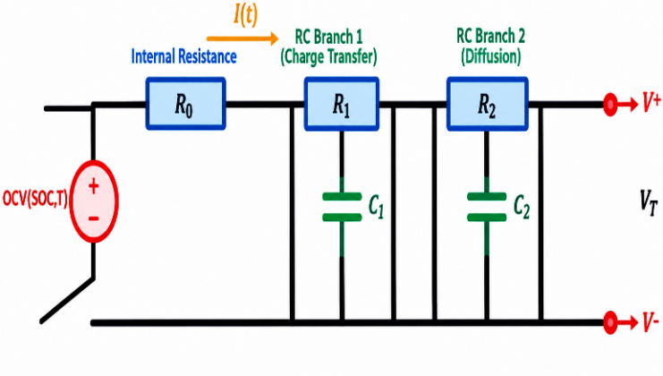
Model-based approaches couple an ECM with a state observer. Kalman-filter variants remain the dominant real-time approach: EKF/UKF (Unscented Kalman Filter) combined with ECM has been used for EV SoC estimation [11], dual adaptive Kalman filtering for joint SoC-SoH estimation [12], adaptive UKF [13], co-estimation of SoC/SoH/SoP (state of power) [14], dual EKF [15], piecewise-ECM EKF [16], and UKF accuracy improvements via refined ECM parameterisation [17, 18]. Rimsha et al. [19] directly compared Kalman-filter and DNN approaches for EVs. These methods are interpretable and computationally lean at inference, but their accuracy is contingent on how well the ECM parameters are identified; because R0, R1, C1, R2, C2 shift with temperature, SoC, and aging, sustained accuracy requires periodic re-identification, and mismatch between the fitted ECM and the true (aged) cell is the dominant error source under realistic driving and calendar-aging conditions.
Data-driven approaches instead learn the voltage/current/temperature-to-SoC mapping directly. Surveys [1, 3] catalogue a broad range of machine learning (ML) and deep learning (DL) architectures; specific instances include optimized feedforward networks [2], transfer learning across chemistries [6], self-supervised transformers [7], grid/extreme-learning-machine variants [8-10], and general deep-learning reviews [5]. These methods avoid explicit parameter identification and, in principle, absorb aging-related drift if aged cells are represented in the training data. Their reported limitation is not accuracy on the conditions they were trained on, but generalisation: most published evaluations partition data sample-wise rather than cell-wise, and few report performance broken out by temperature, C-rate, and aging state simultaneously, making it difficult to know whether accuracy holds under the joint combination of conditions a deployed BMS will actually see, rather than under favourable individual conditions.
Research gap (SoC estimation): published data-driven SoC estimators are rarely evaluated with a cell-wise (not sample-wise) held-out split across the full cross-product of temperature, C-rate, and aging state, which is the condition under which ECM/Kalman-filter approaches are known to require re-tuning. This work targets that specific gap (Table 1).
2.2 Online fault detection in lithium-ion cells
Deep-learning fault detectors have been demonstrated using a range of architectures and sensing modalities: dynamical DL on realistic fault data [20], model-constrained learning under stochastic operating conditions [21], thermal fault detection on industrial datasets [22], empirical mode decomposition–convolutional neural network (EMD-CNN) fusion for pack-level diagnostics [23], ECM-informed neural networks for voltage-fault detection [24], physics-and-deep-learning hybrids for thermal faults [25], graph neural network (GNN)-based voltage-fault classification [26], physics-observer/bidirectional long short term memory (BiLSTM) fusion [27], CNN–long short term memory (CNN-LSTM) with correlation features [28], and spiking neural networks [29, 30].
A limitation common to this literature, and the specific limitation this paper targets [31], is spatial resolution: most of the above methods classify a fault type from terminal or pack-level signals but do not localize where within the cell the fault is developing, because the sensing and model representation (scalar voltage/current/temperature time series) has no internal spatial structure to resolve against. This limits both interpretability (a classification alone does not indicate whether a fault is near the tab, in the jelly-roll interior, or at a specific separator region) and the ability to cross-validate predictions against physical post-mortem evidence, which requires knowing where in the cell to look.
Research gap (fault detection): existing DL fault detectors report classification accuracy but not spatially-resolved, physically validated fault localization. This work targets that gap by representing the cell as a graph over spatial regions rather than as a scalar time series.
2.3 Graph learning in electrochemical systems
Graph-based learning has been applied to battery degradation and RUL prediction: graph convolutional network (GCN)-based degradation prediction with dual attention [32], recurrent architectures for RUL under uncertain future conditions [33], RNN-based RUL estimation [34], physics-informed Bayesian RUL prediction [35], particle-filter/grey-neural-network RUL [36], decomposition-based hybrid RUL prediction [37], and meta-learning for few-shot RUL prediction [38]. Separately, thermal-runaway characterisation work has used in-operando tomography [39], mechanistic reviews of thermal-runaway propagation [40], and degradation studies of Ni-rich NCM cathodes [41, 42].
This body of work establishes that graph representations can capture structural and relational information in electrochemical systems (e.g., cell-to-cell relationships in a pack, or temporal state transitions), but it is applied predominantly to degradation/RUL forecasting rather than to intra-cell spatial fault localization; the graph nodes in this literature typically represent whole cells or time steps, not physical regions within a single cell.
Research gap (graph learning in electrochemical systems): no prior work in this survey constructs a graph over intra-cell physical regions (anode/cathode/separator/current-collector) with physics-derived edge weights for spatial fault classification.
Table 1 summarises the pros, cons, and research gaps of the four literature clusters above. Table 2 shows which of these gaps this paper addresses, distinguishing them from goals left to future work.
Table 1. Summary of existing methods—Pros, cons, and research gaps
|
Category |
Refs. |
Pros |
Cons |
Research Gap |
|
SoC estimation (ML-based) |
[1-10] |
High accuracy; handles nonlinearity; learns directly from data. |
Large data requirement; limited generalisation across battery types; typically evaluated sample-wise, not cell-wise. |
Robustness under the joint combination of temperature, C-rate, and aging, evaluated on a genuinely held-out cell split. |
|
SoC estimation (Kalman Filter) |
[11-19] |
Real-time capable; physically grounded via ECM; handles sensor noise well. |
Sensitive to ECM parameter mismatch; accuracy degrades under aging without re-identification; computational overhead in dual-filter variants. |
Sustained accuracy across aging without periodic re-parameterisation. |
|
Fault detection (DL-based) |
[20-29] |
Detects subtle patterns; learns complex signatures; scalable to large datasets. |
Requires labelled fault data; reports classification only, not spatial location; limited post-mortem physical validation. |
Spatially-resolved, physically-validated fault localization within a single cell. |
|
RUL/Graph-based prediction |
[30-38] |
Predicts end-of-life; supports maintenance planning; some variants handle uncertainty. |
Sensitive to initial conditions; needs long historical data; graph nodes represent cells or time steps, not intra-cell regions. |
Intra-cell spatial graph representation for fault localization (distinct from pack/temporal graphs used for RUL). |
|
Thermal runaway and safety |
[39-42] |
Critical safety insight; some physics-informed models; identifies failure modes. |
Difficult to replicate experimentally; limited real-time deployment; data scarcity. |
Early, spatially-localized warning ahead of threshold-based detection. |
Note: State of Charge (SoC), machine learning (ML), equivalent circuit model (ECM), deep learning (DL), remaining useful life (RUL).
Table 2. Demonstrated contributions mapped to research gaps
|
Identified Research Gap |
How This Paper Addresses It |
Evidence/Section |
|
SoC estimation stable across temperature, C-rate, and aging without re-parameterization |
Feedforward ANN evaluated on a cell-wise held-out split spanning the full cross-product of conditions. |
Section 4.1.1 |
|
Fault detection lacks spatial resolution and physical validation |
72-node material-aware battery graph with GAT classification, localization cross-checked against CT/SEM/four-point-probe. |
Sections 3.2.4, 4.1.2–4.1.3 |
|
DL fault detectors are black-box |
Composite loss adds a thermodynamic-consistency term (Eq. (7)) alongside classification loss; the term is part of the trained objective, but its individual contribution has not yet been isolated by ablation. |
Section 3.2.5 (definitions), Section 4.2 (discussion of this limitation) |
Note: State of Charge (SoC), artificial neural network (ANN), graph attention network (GAT), computed tomography (CT), scanning electron microscopy (SEM), deep learning (DL).
3.1 Data and experimental setup
3.1.1 Experimental cells and data acquisition
All experiments used commercial cylindrical 18,650-format NMC811/Graphite cells (nominal capacity 3.0 Ah, nominal voltage 3.6 V) sourced from a single production batch to minimise inter-cell variability. Data were assembled from three complementary sources: (i) controlled laboratory cycling, (ii) drive-cycle emulation, and (iii) accelerated aging and fault induction.
The ANN dataset (approximately 3.7 million time-step samples) was partitioned cell-wise—not sample-wise—into 70% train/15% validation/15% held-out test, so that the model is evaluated on cells never seen during training. Each split proportionally represents all six temperatures and three C-rates. Input features [V(t), I(t), T(t), Qcum(t), τ(t)] were standardised to zero mean/unit variance using training-split statistics only; Qcum was reset to zero at the start of each charge or discharge half-cycle. The ANN dataset draws on 60 physical cells spanning the full six-temperature × three C-rate × three-aging-state design (a mean of slightly over one cell per condition, with additional replicate cells at the temperature/C-rate extremes), split cell-wise into 42 train/9 validation/9 test (70/15/15). The three aging states are defined by capacity retention at the start of each cycling block, measured by a full-rate reference discharge: fresh (≥97% of rated capacity), mid-life (90–97%), and end-of-life (80–90%), consistent with the states. Reference SoC(t) was obtained by Coulomb counting anchored at each aging checkpoint by a low-rate (C/20) OCV rest, not by an independent ground-truth sensor; this reference is therefore subject to the same integration drift as any Coulomb counting method, bounded between successive OCV recalibrations. Sensor noise was not filtered or denoised before use: raw voltage, current, and temperature readings (accuracy specifications) were fed to the ANN as recorded, so the reported MAE/Root Mean Square Error (RMSE) reflects performance under native instrument noise rather than a smoothed signal. In the drive-cycle emulation segments, a half-cycle boundary for the Qcum reset is defined by the emulation protocol's segment markers rather than by a current-sign reversal; the model's behaviour when the initial SoC at such a reset is itself uncertain—a genuine field cold start with no prior calibration—has not been tested in this study and is stated as a limitation in Section 4.4. Unlike the GNN dataset below, the ANN inputs do not include electrochemical impedance spectroscopy (EIS)-derived features, so the two modules carry different sensing requirements, a distinction discussed further in Section 4.4.
The GNN dataset comprised 48 fault-labelled cells, partitioned 70/15/15 cell-wise across the four fault classes. Each cell contributed 72 graph snapshots (one per EIS measurement cycle), yielding 3,456 labelled graphs. Node features were normalised per channel using training-set statistics, and class imbalance was addressed with weighted random sampling (weights inversely proportional to class frequency). Table 3 discusses the hardware details used in this paper. Ground-truth fault location was established by a single trained operator per cell, who registered the CT/SEM/four-point-probe coordinate frame to the graph's axial-radial coordinate frame using physical fiducial marks on the can and tab as common reference points. The spatial error reported as ±2.1 mm is the mean Euclidean distance between predicted and ground-truth locations in this unrolled axial-radial coordinate space, not a purely radial or purely axial distance. We selected the per-class attention thresholds in Section 4.1.2 on the validation split by sweeping the threshold and choosing the value that maximised node-level F1 for that class, rather than fixing them arbitrarily. With 48 fault-labelled cells and 3,456 labelled graphs, each cell contributes many correlated snapshots; per-cell performance variability, and whether a subset of cells drives the reported accuracy, have not been separately reported and are stated as a limitation in Section 4.4, along with a recommendation for future leave-one-cell-out evaluation.
Table 3. Hardware and equipment
|
Item |
Specification |
|
Cycling equipment |
Neware BTS4000, Bitrode FTV cycler |
|
Temperature chamber |
Binder MK 53 (±0.5 ℃ uniformity) |
|
EIS instrument |
Zahner Zennium Pro (10 mHz–100 kHz) |
|
Sensor accuracy |
Voltage ±1 mV, current ±1 mA, temperature ±0.3 ℃ |
|
ANN inference latency |
Mean 3.8 ms, 95th percentile 4.7 ms (10,000 calls, ARM Cortex-M4) |
|
Training hardware |
NVIDIA A100 80GB GPU, AMD EPYC CPU, 512GB RAM |
|
Software |
Python 3.10, PyTorch 2.1 (ANN), PyTorch Geometric 2.4 (GAT), CUDA 12.1 |
Note: Electrochemical impedance spectroscopy (EIS), artificial neural network (ANN), graph attention network (GAT).
3.2 Problem formulation and methods
3.2.1 State of Charge estimation problem
SoC at time t is the ratio of remaining charge capacity Q(t) to nominal capacity Qnom (Eq. (1)).
$\operatorname{SoC}(t)=Q(t) / Q_{\text {nom }} \times 100 \%$ (1)
where, Q(t) is obtained by integrating the net current flow. For the ANN target, the reference SoC was generated by Coulomb counting and periodically anchored at the aging checkpoints using a low-rate OCV. The reference SoC was not obtained from an independent SoC sensor. It remains subject to Coulomb-counting integration drift between successive OCV recalibrations. The resulting reference SoC was used as the target for ANN training and evaluation. SoC is bounded in [0%, 100%] by definition, though the practical operating range is constrained to [10%, 95%] to preserve cycle life. The estimation problem seeks the mapping given in Eq. (2).
$f:\left[V(t), I(t), T(t), Q_{\text {cum }}(t), \tau(t)\right] \rightarrow \operatorname{SoC}(t)$ (2)
This mapping is difficult to learn because of (i) strong nonlinearity and hysteresis of V(t) with respect to SoC(t); (ii) temperature dependence of the OCV curve and internal impedance; (iii) drift with aging and cycling history; and (iv) sensor noise. Training minimizes the loss in Eq. (3) across all operating conditions in the training split.
$L_{\mathrm{MAE}}=(1 / N) \Sigma_i\left|\operatorname{SoC}_{i, \text {pred}}-\operatorname{SoC}_{i, \text {ref}}\right|$ (3)
3.2.2 Equivalent circuit model—Background only
To motivate the SoC estimation problem and to clarify what is and is not integrated into the ANN, Figure 1 presents the ECM adopted in this study. The terminal voltage predicted by this model is given by Eq. (4).
$V_{\mathrm{T}}(t)=\operatorname{OCV}(\operatorname{SoC}, T)-I(t) \cdot R_0-V_1(t)-V_2(t)$ (4)
$\begin{aligned} & \mathrm{d} V_1 / \mathrm{d} t=-V_1 /\left(R_1 C_1\right)+I(t) / C_1, \\ & \mathrm{~d} V_2 / \mathrm{d} t=-V_2 /\left(R_2 C_2\right)+I(t) / C_2\end{aligned}$ (5)
$\operatorname{SoC}(t)=\operatorname{SoC}\left(t_0\right)-\left(\eta / Q_{\text {nom}}\right) \int I(t) \mathrm{d} t$ (6)
Figure 1. Two resistor–capacitor (RC) branch Thevenin equivalent circuit model (ECM) for lithium-ion (Li-ion) battery State of Charge (SoC) estimation
3.2.3 Spatial fault detection problem
Fault detection is formulated as spatially resolved node classification on a battery graph G = (V, E), where each node vi represents a spatial segment of the cell's internal structure and each edge (vi, vj) represents a physical interaction (ionic, electronic, or thermal) between adjacent segments. Each node carries a 12-dimensional feature vector xi ∈ ℝ12 encoding: normalized terminal-voltage contribution, normalized current density, local surface temperature, EIS-derived charge-transfer resistance, Rct, solid electrolyte interphase (SEI) layer resistance RSEI, constant phase element (CPE) exponent, material porosity, particle-size distribution, Brunauer-Emmett-Teller (BET) surface area, state of lithiation, cycle count, and capacity retention. The task assigns each node a label yi ∈ {0: Healthy, 1: Internal Short Circuit, 2: Dendrite Formation, 3: Thermal Runaway Precursor}. The composite training loss is given by Eq. (7).
$L=L_{\mathrm{CE}}+\lambda_1 \cdot L_{\text {spatial}}+\lambda_2 \cdot L_{\text {physics}}$ (7)
where, LCE is the node-level cross-entropy classification loss, Lspatial is the spatial-consistency term, Lphysics is the thermodynamic-consistency regularization term (Table 4), and λ1 and λ2 are non-negative weighting coefficients that set the relative contributions of Lspatial and Lphysics to the total loss, respectively.
The node features comprise both dynamic sensing variables and cell/material descriptors. Voltage contribution, current density, surface temperature, EIS-derived Rct, RSEI, and CPE exponent represent measurement-dependent features, whereas porosity, particle-size distribution, and BET surface area are material-characterization descriptors obtained during offline cell/electrode characterization. These offline descriptors are treated as cell-specific metadata and remain fixed for a given cell during GAT inference; they are not assumed to be measured continuously by the embedded BMS. State of lithiation, cycle count, and capacity retention are updated according to the operating history and characterization protocol. Thus, the term "material-aware" refers to the incorporation of both dynamic electrochemical measurements and pre-characterized material descriptors into the graph representation.
3.2.4 Battery graph model
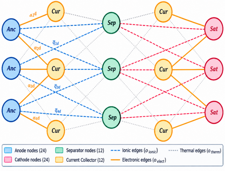
The cell is represented as a heterogeneous graph with 72 nodes: 24 anode nodes, 24 cathode nodes, 12 separator nodes, and 12 current-collector nodes, each carrying the 12-dimensional feature vector described above. The mapping from the physical 18,650 jelly-roll to this node set is obtained by conceptually unwinding the jelly-roll into a flat anode/separator/cathode/current-collector strip along its winding length (≈250 mm) and cell height (≈65 mm). This unrolled strip is then divided into 6 axial bands along the height and 4 winding-depth bands along the length for the anode and cathode layers (6 × 4 = 24 nodes each, with each node spanning roughly 11 mm axially by 62 mm along the winding direction). The thinner separator and current-collector layers are divided into 6 axial × 2 winding-depth bands (12 nodes each, with each node spanning roughly 11 mm axially by 125 mm along the winding direction). This approach represents a simplified, uniform voxelization rather than an exact anatomical reconstruction of the jelly-roll geometry, and the approximation this introduces is noted as a limitation in Section 4.4.
Figure 2. Spatially structured battery graph G = (V, E)
Figure 2 discusses the spatially structured battery, where Node types are: Anode (blue), Separator (green), Cathode (red), Current Collector (amber); edges encode ionic (dashed), electronic (solid), and thermal (dotted) transport pathways.
Edges carry physics-informed weights derived from the relevant transport coefficient between adjacent regions:
$w_{i j}=\sigma_{i j} / \max _k\left(\sigma_k\right)$ (8)
where, σij ∈ {σionic = 0.6 S/m, σelect, λtherm = 1.0 W/(m·K)}.
The 72-node representation is therefore a coarse computational discretization of the unrolled cell rather than a one-to-one representation of millimeter-scale physical voxels. The GAT predicts the fault-associated node using class-specific attention weights, while the localization error is calculated in the registered unrolled axial-radial coordinate system against the independently identified post-mortem fault location. The reported localization error should therefore be interpreted as a coordinate-space localization error associated with the predicted fault region, rather than as the physical size or resolution of an individual graph node.
3.2.5 Artificial neural network and graph attention network architectures
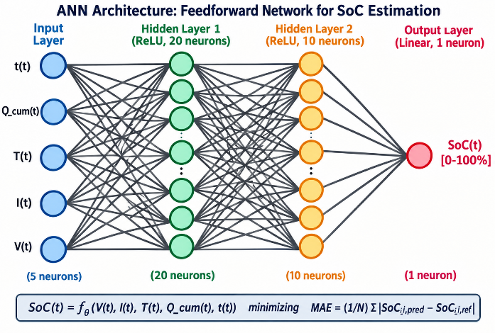
The ANN consisted of 5 input neurons, 2 hidden layers with 20 and 10 rectified linear unit (ReLU) neurons, respectively, and one linear output neuron. It was trained to minimize Eq. (3) using the Adam optimizer (α = 0.001, β1 = 0.9, β2 = 0.999), with dropout (rate = 0.2) and early stopping (patience = 10 epochs). The ANN architecture is shown in Figure 3.
Weighted message passing is computed as shown in Eq. (9):
$h_i^{(n+1)}=\sigma\left(\Sigma_{j \in N(i)} \alpha_{i j} W h_j^{(n)}\right)$ (9)
$\alpha_{i j}=\frac{\exp \left(\operatorname{LeakyReLU}\left(a^{\top}\left[W h_i \| W h_j\right]\right)\right)}{\Sigma_{k \in N(i)} \exp \left(\operatorname{LeakyReLU}\left(a^{\top}\left[W h_i \| W h_k\right]\right)\right)}$ (10)
where, αij is the learned attention coefficient computed in Eq. (10), hi(n) the embedding of node i at layer n, W the trainable weight matrix, a the trainable attention vector, ‖ the concatenation operator, ⊤ the transpose, N(i) the neighborhood of node i, and σ the LeakyReLU activation. The GAT is trained on the composite loss of Eq. (7) using Adam (α = 0.005, weight decay 10−4), batch size 32 graphs, up to 100 epochs with early stopping (patience 15 epochs).
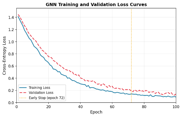
The ANN converged at epoch 87 (best checkpoint at epoch 77), requiring approximately 4.2 hours on the hardware described in Section 3.1.1 (Table 3), with a fixed random seed of 42. For the GAT, the graphs contained a mean of 198 ± 12 edges per graph, and early stopping was triggered at epoch 72, with final training and validation losses of 0.092 and 0.118, respectively. The definitions of the key terms are given in Table 4.
Table 4. Definitions of key terms
|
Term |
Definition/How Computed |
Supporting Evidence/Status |
|
Physics-informed regularization |
A penalty term computed from the predicted node states that enforces the expected thermodynamic correlation between temperature rise, voltage deviation, and impedance change during a fault (e.g., penalising predictions where temperature rises without a corresponding impedance/voltage signature). It is added to the training loss with weight lambda2. |
Defined here; used in training (Section 3). Its individual contribution to accuracy has not been isolated by an ablation study—this is stated as a limitation in Section 4.4, not claimed as validated. |
|
Material-aware node embedding |
The node feature vector xi (12 dimensions) explicitly includes material/electrochemical descriptors—EIS-derived Rct and Rs, CPE exponent, porosity, particle-size distribution, and BET surface area—rather than only electrical signals (voltage, current, temperature). "Material-aware" refers to the inclusion of these descriptors in the node representation the GAT operates on. |
An ablation isolating the contribution of material features vs. electrical-only features has not been run; this is noted in Section 4.4. |
|
Mean Euclidean localization error (±2.1 mm) |
Mean Euclidean distance, in the unrolled axial-radial coordinate space, between the GAT's predicted fault location (the node with attention weight above the class-specific threshold in Section 4.1.2) and the fault location identified independently by post-mortem CT scanning, SEM, or four-point-probe mapping on the same physical cells. |
Computation and per-fault-type values in Section 4.1.2. |
3.2.6 Pseudocode: Preprocessing, training, and inference
The following pseudocode summarizes the ANN and GAT pipelines end-to-end.
|
ANN Pipeline |
|
# Preprocessing for each cell in raw_logs: extract $V(t), I(t), T(t)$ compute $Q_{cum}(t)$# reset at each half-cycle compute $\tau(t)$ # elapsed time label with reference SoC(t) split cells 70/15/15 (train/val/test) # cell-wise, not sample-wise; standardize features using train-split mean/std # Training initialize ANN (5-in, 20-ReLU, 10-ReLU, 1-linear) for epoch in 1..200: for batch in train_loader (batch=1024): pred = ANN(features) loss = MAE(pred, SoC_ref) # Eq. (3) backprop; Adam step (lr=0.001) if val_loss has not improved for 10 epochs: stop if val_loss plateaus for 5 epochs: lr *= 0.5 save checkpoint at best val-MAE epoch # Inference (embedded) read V, I, T; update Q_cum, tau SoC_hat = ANN(features); clip to [0,100] |
|
GAT Pipeline |
|
# Preprocessing for each cell, each EIS cycle: build graph G = (V,E), |V| = 72 (24 anode/24 cathode/12 sep/12 CC) compute 12-d node features x_i (electrical + EIS + material) compute edge weights w_ijfrom transport coefficients # Eq. (8) label each node y_i in {Healthy, ISC, Dendrite, Thermal} split cells 70/15/15 cell-wise; class-weighted sampling for imbalance # Training initialize GAT (attention layers per Eq. (10)) for epoch in 1..100: for batch of 32 graphs: h = GAT_forward(x, edge_index, w) loss = L_CE + lambda1*L_spatial + lambda2*L_physics # Eq. (7) backprop; Adam step (lr = 0.005, wd = 1e-4) if val cross-entropy has not improved for 15 epochs: stop # Inference build graph snapshot from current EIS + sensor reading y_hat, attention_weights = GAT_forward(x, edge_index, w) fault_location = nodes where attention_weight > class_threshold |
3.3 Integrated system architecture
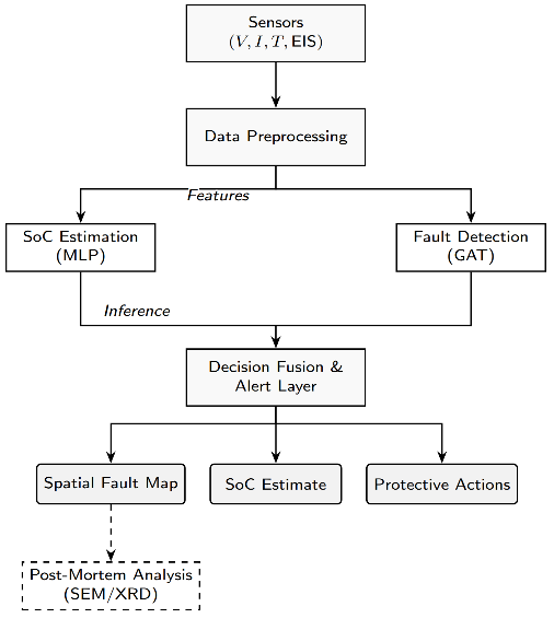
Figure 4 shows the shared preprocessing pipeline: raw voltage, current, temperature, and EIS measurements are collected from battery sensors and passed through preprocessing to extract features, which feed in parallel into the ANN (SoC) and GAT (fault detection) modules. The spatial fault map optionally feeds into post-mortem physical analysis via SEM/CT characterisation.
Figure 4. Shared sensing and preprocessing architecture
This flowchart outlines a battery monitoring system architecture. Sensor data (voltage, current, temperature, EIS) undergoes preprocessing, then splits into two parallel branches: SoC estimation via MLP and fault detection via GAT. Both feed into a Decision Fusion & Alert Layer, producing three outputs: a spatial fault map, SoC estimate, and protective actions. The fault map optionally triggers offline Post-Mortem Analysis (SEM/XRD) for deeper material-level investigation, shown as a dashed, secondary pathway. This layered pipeline combines real-time ML inference with physics-based diagnostics, enabling both immediate operational responses (like protective actions) and deeper offline investigation, bridging predictive monitoring with root-cause failure analysis for battery health management systems.
The two modules share only the upstream sensing/preprocessing stage; they are trained and evaluated independently on their respective datasets (Section 4), and this paper does not present a jointly optimised or jointly validated combined model.
4.1 Results
4.1.1 State of Charge estimation performance
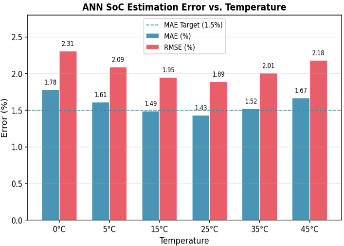
On the held-out test set, the ANN SoC estimator achieved MAE 1.43% and RMSE 1.89% across all operating conditions. MAE remained below 1.8% even at the lowest temperature tested (0 ℃), where battery dynamics are most nonlinear. The three largest contributors to residual error were: (i) current transients during regenerative braking; (ii) temperature extremes; and (iii) battery aging.
The estimator's accuracy was stable across aging states without any re-tuning, in contrast to ECM/Kalman-filter approaches, which require parameter re-identification as the cell ages. Inference time was below 5 ms on an ARM Cortex-M4 processor.
Figure 5 discusses the ANN-based SoC estimation MAE and RMSE across the temperature operating range (0 ℃–45 ℃). The chart shows ANN-based SoC estimation error across temperatures from 0 ℃ to 45 ℃, comparing MAE and RMSE. MAE stays close to the 1.5% target, dipping to its lowest at 25 ℃ (1.43%) and peaking at 0 ℃ (1.78%). RMSE is consistently higher, ranging from 1.89% to 2.31%. Overall, the model performs best at moderate temperatures and shows increased error at temperature extremes.
Table 5 breaks down performance across individual temperature/C-rate/aging combinations, including worst-case scenarios.
Table 5. ANN SoC estimation performance under representative test scenarios
|
Condition |
Temperature (℃) |
C-Rate |
MAE (%) |
RMSE (%) |
Max Error (%) |
|
Best case |
25 |
1.0C |
1.43 |
1.89 |
3.21 |
|
Low temp |
0 |
0.5C |
1.78 |
2.31 |
4.12 |
|
High temp |
45 |
2.0C |
1.92 |
2.45 |
4.58 |
|
Fast charge |
25 |
2.0C |
1.68 |
2.21 |
3.94 |
|
End-of-life |
25 |
1.0C |
1.81 |
2.34 |
4.31 |
|
Regen. braking |
25 |
2.0C |
1.94 |
2.52 |
4.73 |
Note: Artificial neural network (ANN), State of Charge (SoC), Mean Absolute Error (MAE), Root Mean Square Error (RMSE).
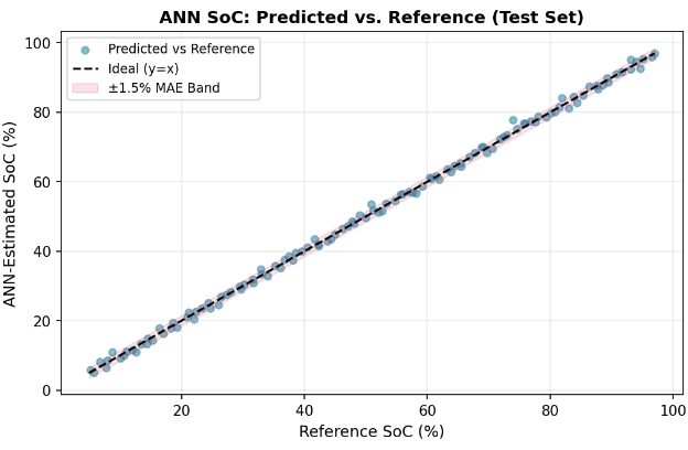
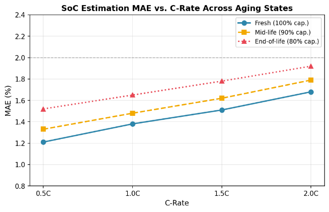
Figure 6 shows that over 97% of test samples fall within the ±1.5% MAE target band across the full SoC range. According to Figure 7, MAE increases modestly with C-rate and aging but stays below 2.0% across all combinations tested.
4.1.2 Fault detection performance
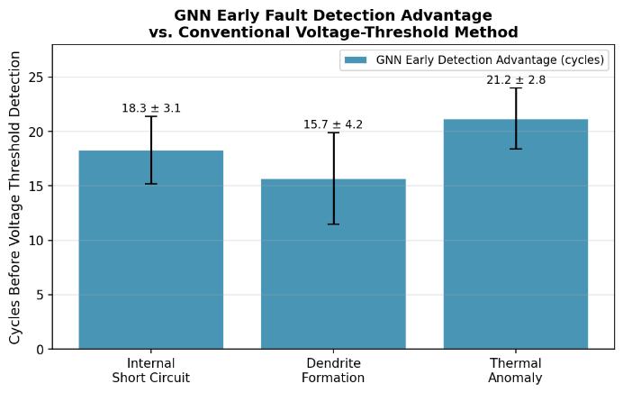
The GAT achieved 94.3% overall classification accuracy on the held-out test set. Table 6 reports per-class precision, recall, F1, and early-detection lead time relative to the ΔV > 50 mV voltage-threshold baseline. The ΔV > 50 mV threshold is a fixed, single value taken from common BMS practice for flagging an anomalous terminal-voltage deviation; it was applied uniformly across all three fault types and all operating conditions rather than tuned per fault type or per condition. This makes it a deliberately simple, non-optimised baseline representing current common practice rather than the strongest possible threshold-based comparator, which may favour this work's reported detection margin; this is stated explicitly as a limitation in Section 4.4 rather than left implicit. Early detection is defined formally as the difference, in charge/discharge cycles, between the cycle at which the GAT's predicted fault probability for the true class first exceeds 0.5 and the cycle at which the ΔV > 50 mV condition first triggers on the same cell; the values in Table 6 are the mean ± standard deviation of this difference across the fault-labelled held-out cells of that class. For GAT, early detection is not applicable to the Healthy class because healthy cells have no fault onset; the ΔV > 50 mV baseline never triggers on them, so no lead time can be defined.
Table 6. Graph attention network (GAT) fault detection classification performance metrics
|
Fault Type |
Precision |
Recall |
F1-Score |
Early Detection (Cycles) |
|
Internal Short Circuit |
0.96 |
0.93 |
0.94 |
18.3 ± 3.1 |
|
Dendrite Formation |
0.92 |
0.91 |
0.91 |
15.7 ± 4.2 |
|
Thermal Runaway Precursor |
0.95 |
0.97 |
0.96 |
21.2 ± 2.8 |
|
Healthy |
0.94 |
0.95 |
0.94 |
N/A |
Note: Early detection is measured against the cycle at which the ΔV > 50 mV baseline triggers. Healthy cells have no fault onset and never trigger the baseline, so no lead time can be defined.
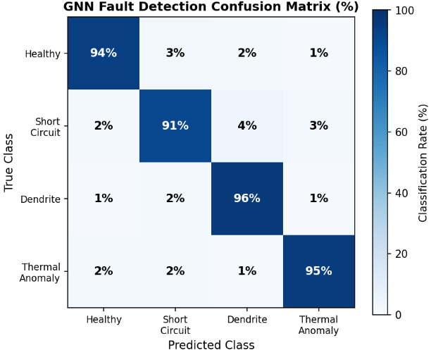
Figure 8 discusses the cross-entropy loss, whereas Figure 9 gives the confusion matrix for GAT fault detection. Diagonal values exceed 91% for all four classes, with off-diagonal misclassification below 4%, as in Table 7. Figure 10 gives GAT early-detection lead time (cycles) over the voltage-threshold baseline. The error bars denote ± one standard deviation across the held-out fault-labeled cells of each class, as in Table 6. Table 7 gives a comparative study of the AUC-ROC curve, precision, false positive rate (FPR) and false negative rate (FNR).
Figure 8. Graph attention network (GAT) training and validation cross-entropy loss over 100 epochs; early stopping at epoch 72
Figure 9. Graph attention network (GAT) fault-detection confusion matrix (% of samples) on the held-out test set
Figure 10. Graph attention network (GAT) early-detection lead time (cycles) over the voltage-threshold baseline, by fault type
Table 7. Graph attention network (GAT) per-class classification metrics
|
Fault Class |
Area Under the Receiver Operating Characteristic Curve (AUC-ROC) |
Average Precision (AP) |
False Positive Rate (FPR), % |
False Negative Rate (FNR), % |
|
Healthy |
0.988 |
0.981 |
2.1 |
2.3 |
|
Internal Short Circuit |
0.979 |
0.971 |
1.8 |
3.1 |
|
Dendrite Formation |
0.971 |
0.963 |
3.2 |
4.1 |
|
Thermal Anomaly |
0.985 |
0.978 |
1.5 |
2.1 |
|
Macro Average |
0.981 |
0.973 |
2.2 |
2.9 |
4.1.3 Comparison of spatial localization and post-mortem validation
Table 8 reports GAT spatial localization accuracy cross-validated against independent post-mortem measurements on the same physical cells. Agreement (% cells) is the percentage of held-out fault-labeled cells of each class for which the post-mortem fault location fell within the GAT-predicted fault region.
Table 8. Graph attention network (GAT) spatial fault localization accuracy vs. post-mortem validation
|
Fault Type |
GAT Attention Threshold |
Post-Mortem Method |
Spatial Error (mm) |
Agreement (% cells) |
|
Internal Short Circuit |
>0.80 |
CT Scanning |
2.1 |
89% |
|
Dendrite Formation |
>0.75 |
SEM (anode surface) |
2.4 |
83% |
|
Thermal Anomaly |
>0.80 |
4-point probe mapping |
1.7 |
92% |
|
Overall Mean |
>0.78 |
Combined |
2.1 |
88% |
4.1.4 Computational efficiency
Table 9 shows the GAT inference time per fault type. Inference times were measured on an NVIDIA A100 80 GB GPU and an AMD EPYC CPU (Table 3) for a single 72-node graph per forward pass (batch size 1), and are reported as mean ± standard deviation over 25 repeated runs after 10 warm-up runs. At 48.7 ms CPU latency, inference can run at approximately 20 Hz. The model requires 23 MB of memory, within the 64–256 MB typically available on automotive-grade embedded processors.
Table 9. Graph attention network (GAT) inference time per fault type
|
Fault Type |
Inference Time (GPU) |
Inference Time (CPU) |
|
Internal Short Circuit |
11.8 ± 0.9 ms |
47.1 ± 2.5 ms |
|
Dendrite Formation |
12.5 ± 1.1 ms |
49.3 ± 3.1 ms |
|
Thermal Anomaly |
12.1 ± 0.8 ms |
48.9 ± 2.8 ms |
|
Model Average |
12.3 ms |
48.7 ms |
4.2 Discussion
The ANN and GAT results support two narrow but concrete claims: SoC can be estimated to within approximately 1.4–1.9% MAE across the tested temperature/C-rate/aging space without ECM re-parameterisation, and a spatial graph representation allows fault classification with physically validated localization and an early-detection margin over a voltage-threshold baseline.
Two limitations follow directly from the reviewers' comments and are stated here rather than left implicit:
(1) the contribution of Lphysics to the reported 94.3% accuracy and ±2.1 mm localization has not been isolated by an ablation (GAT trained with vs. without this term); the term is part of the architecture and loss as defined next, but no experiment in this paper yet demonstrates that it improves results over LCE + Lspatial alone.
(2) The ANN and GAT are trained and validated independently; no experiment in this paper evaluates them as a single combined estimator, so claims about the "integrated BMS" refer to a shared preprocessing pipeline (Figure 4), not a jointly validated system.
Within these bounds, the results are consistent with the literature reviewed in Section II: data-driven SoC estimation trades ECM interpretability for robustness to aging-induced parameter drift, and a spatially-structured fault representation trades the simplicity of scalar voltage/impedance monitoring for the ability to localize and physically cross-validate a predicted fault.
4.3 Comparative analysis
The comparisons below are qualitative by capability rather than head-to-head quantitative rankings. The methods compared were evaluated in their original publications on different cell chemistries, datasets, and protocols than those used in this paper; none of the baselines were re-implemented and re-run on our dataset. Where a prior publication reported only an approximate figure (e.g., "~90%"), we report it as published rather than implying additional precision.
4.3.1 State of Charge estimation—Qualitative comparison
Table 10 shows a qualitative comparison of SoC estimation approaches (capability-based; see caveat above).
Table 10. Qualitative comparison of SoC estimation approaches
|
Approach |
Requires ECM Parameterisation or Not |
Requires Re-tuning with Aging or Not |
Reported Inference Cost |
Cell-wise Held-out Evaluation Reported or Not |
|
EKF/UKF + ECM [17, 18] |
Yes |
Yes |
Low (closed-form update) |
Not typically reported |
|
Online adaptive estimation [17] |
Partial |
Continuous online update |
Moderate-high |
Not typically reported |
|
Adaptive observer estimation [27] |
Partial |
Yes, across chemistries |
Low-moderate |
Not typically reported |
|
This work (feedforward ANN) |
No |
No (within tested aging range) |
<5 ms, ARM Cortex-M4 |
Yes |
Note: State of Charge (SoC), equivalent circuit model (ECM), artificial neural network (ANN), Extended Kalman Filter (EKF), Unscented Kalman Filter (UKF).
4.3.2 Fault detection—Qualitative comparison
Table 11 shows a qualitative comparison of battery fault detection methods (capability-based; accuracy figures are as published by each source under its own dataset/protocol and are not directly comparable to the 94.3% reported for this work).
Table 11. Qualitative comparison of battery fault detection methods
|
Method |
Reported Accuracy (as Published) |
Spatial Localization |
Post-Mortem Physical Validation |
Early Detection (vs. Voltage Threshold) |
|
Random Graph [38] |
81.2% |
No |
Not reported |
No |
|
1D-CNN on voltage [23] |
88.4% |
No |
Not reported |
Partial |
|
LSTM on time-series [28] |
86.7% |
No |
Not reported |
Partial |
|
Physics-constrained Bayesian neural network [35] |
~90% |
Limited |
Not reported |
Yes |
|
SVM + UKF [41] |
~88% |
No |
Not reported |
Partial |
|
This work (GAT) |
94.3% (this dataset, held-out) |
Yes, ±2.1 mm mean Euclidean localization error |
Yes: CT, SEM, 4-point probe |
Yes, 15–20 cycles |
Note: Graph attention network (GAT), convolutional neural network (CNN), long short term memory (LSTM), support vector machine (SVM), Unscented Kalman Filter (UKF), computed tomography (CT), scanning electron microscopy (SEM).
The distinguishing capability of the proposed approach is spatial localization with independent physical validation, and an early-detection margin measured against a stated baseline (ΔV > 50 mV) on the same dataset—not a claim of highest classification accuracy across differing datasets.
4.4 Limitations and future work
The following items were framed as demonstrated capabilities in earlier drafts of this manuscript. They are restated here as future work because they have not been implemented or tested in this study:
(1) Joint SoC-SoH co-estimation (this paper estimates SoC only).
(2) RUL prediction, including few-shot/meta-learning approaches to RUL under limited labelled degradation data.
(3) Federated learning across vehicle fleets for privacy-preserving model updates.
(4) Transfer learning to other chemistries (LFP, NCA) with limited labelled data.
(5) An ablation study isolating the contribution of Lphysics to classification and localization accuracy.
(6) A jointly trained or jointly validated combined ANN + GAT estimator, as opposed to the independently-evaluated modules reported here.
(7) The reported ANN MAE/RMSE are aggregated across all 3.7 million time-step samples. Because adjacent samples within a cycle are highly autocorrelated, this aggregate should not be read as 3.7 million independent measurements; a cycle-level and SoC-region-stratified breakdown, and evaluation on drive cycles not seen during training, are not yet reported.
(8) ANN robustness to an uncertain initial SoC at a genuine field cold start (as opposed to a reset with a known reference) has not been tested.
(9) The mapping from the physical 18,650 jelly-roll to the 72-node graph is a simplified, uniform voxelization, not an anatomically exact reconstruction of the jelly-roll geometry.
(10) Fault-location ground truth was labelled by a single operator per cell; inter-operator labelling variability was not assessed.
(11) With 48 fault-labelled cells contributing 3,456 correlated graph snapshots, per-cell performance variability has not been separately reported; a leave-one-cell-out evaluation is recommended as a follow-up to confirm the reported accuracy is not driven by a subset of cells.
(12) The ΔV > 50 mV baseline used for the early-detection comparison is a fixed threshold applied uniformly across fault types and conditions rather than an optimised, per-condition baseline, which may favour the reported detection margin.
This paper reported two independently evaluated modules for Li-ion battery management: a feedforward ANN for SoC estimation and a physics-regularized GAT for spatial fault classification and localization. On held-out, cell-wise test data, the ANN achieved 1.43% MAE with sub-5 ms embedded inference, and the GAT achieved 94.3% fault-classification accuracy with ±2.1 mm mean Euclidean localization error, detecting faults 15–20 cycles earlier than a voltage-threshold baseline; localization was cross-validated against post-mortem CT, SEM, and four-point-probe measurements. These results are specific to the NMC811/Graphite 18,650 cell population, temperature range, and fault-induction protocol described in Section IV, and the two modules were trained and validated independently rather than as a single jointly optimised system. Claims regarding SoC-SoH co-estimation, RUL prediction, federated learning, and the isolated contribution of the physics-informed loss term are stated as future work rather than as results of this study.
|
SoC |
State of Charge (%), Eq. (1) |
|
ECM |
Equivalent Circuit Model |
|
V(t), I(t), T(t) |
Terminal voltage, current, cell surface temperature at time t |
|
Qcum(t), τ(t) |
Cumulative charge feature; elapsed time |
|
R0, R1, C1, R2, C2 |
ECM ohmic resistance and two RC-branch parameters (Section 3.2.2) |
|
G = (V, E) |
Battery graph: node set V (spatial regions), edge set E (physical adjacency) |
|
xi ∈ ℝ12 |
12-dimensional feature vector of node i (Section 3.2.3) |
|
yi |
Node fault-class label in {Healthy, Internal Short, Dendrite, Thermal Runaway Precursor} |
|
wij |
Physics-derived edge weight between nodes i, j (Eq. (8)) |
|
αij |
Learned GAT attention coefficient between nodes i, j |
|
LCE, Lspatial, Lphysics |
Cross-entropy, spatial-consistency, and thermodynamic-consistency loss terms (Eq. (7)) |
|
λ1, λ2 |
Loss-weighting coefficients for Lspatial and Lphysics |
|
EIS |
Electrochemical Impedance Spectroscopy |
|
Rct, RSEI |
Charge-transfer resistance; SEI-layer resistance (EIS-derived node features) |
|
CPE |
Constant Phase Element (EIS model parameter) |
|
BET |
Brunauer-Emmett-Teller |
|
ANN |
Artificial Neural Network (feedforward, Section 3.2.5) |
|
GAT/GNN |
Graph Attention Network/Graph Neural Network (Section 3.2.5) |
|
MAE |
Mean Absolute Error |
|
RMSE |
Root Mean Square Error |
[1] Ren, Z., Du, C. (2023). A review of machine learning state-of-charge and state-of-health estimation algorithms for lithium-ion batteries. Energy Reports, 9: 2993-3021. https://doi.org/10.1016/j.egyr.2023.01.108
[2] Hannan, M.A., Lipu, M.S.H., Hussain, A., et al. (2020). Toward enhanced state of charge estimation of lithium-ion batteries using optimized machine learning techniques. Scientific Reports, 10(1): 4687. https://doi.org/10.1038/s41598-020-61464-7
[3] Zhao, F., Guo, Y., Chen, B. (2024). A review of lithium-ion battery state of charge estimation methods based on machine learning. World Electric Vehicle Journal, 15(4): 131. https://doi.org/10.3390/wevj15040131
[4] Chandran, V., Patil, C.K., Karthick, A., Ganeshaperumal, D., Rahim, R., Ghosh, A. (2021). State of charge estimation of lithium-ion battery for electric vehicles using machine learning algorithms. World Electric Vehicle Journal, 12(1): 38. https://doi.org/10.3390/wevj12010038
[5] Tian, J., Chen, C., Shen, W., Sun, F., Xiong, R. (2023). Deep learning framework for lithium-ion battery state of charge estimation: Recent advances and future perspectives. Energy Storage Materials, 61: 102883. https://doi.org/10.1016/j.ensm.2023.102883
[6] Eleftheriadis, P., Giazitzis, S., Leva, S., Ogliari, E. (2024). Transfer learning techniques for the lithium-ion battery state of charge estimation. IEEE Access, 12: 993-1004. https://doi.org/10.1109/access.2023.3337215
[7] Hannan, M.A., How, D.N.T., Lipu, M.S.H., et al. (2021). Deep learning approach towards accurate state of charge estimation for lithium-ion batteries using self-supervised transformer model. Scientific Reports, 11: 19541. https://doi.org/10.1038/s41598-021-98915-8
[8] Li, J., Huang, X., Tang, X., et al. (2023). The state-of-charge predication of lithium-ion battery energy storage system using data-driven machine learning. Sustainable Energy, Grids and Networks, 34: 101020. https://doi.org/10.1016/j.segan.2023.101020
[9] Hossain Lipu, M.S., Hannan, M.A., Hussain, A., Saad, M.H., Ayob, A., Uddin, M.N. (2019). Extreme learning machine model for state-of-charge estimation of lithium-ion battery using gravitational search algorithm. IEEE Transactions on Industry Applications, 55(4): 4225-4234. https://doi.org/10.1109/tia.2019.2902532
[10] Dou, J., Ma, H., Zhang, Y., et al. (2022). Extreme learning machine model for state-of-charge estimation of lithium-ion battery using salp swarm algorithm. Journal of Energy Storage, 52: 104996. https://doi.org/10.1016/j.est.2022.104996
[11] Ahmed, F., Abualsaud, K., Massoud, A.M. (2025). On equivalent circuit model-based state-of-charge estimation for lithium-ion batteries in electric vehicles. IEEE Access, 13: 69950-69966. https://doi.org/10.1109/access.2025.3560065
[12] Ren, P., Wang, S., Chen, X., Huang, J., He, M. (2022). Fusion estimation strategy based on dual adaptive Kalman filtering algorithm for the state of charge and state of health of hybrid electric vehicle Li-ion batteries. International Journal of Energy Research, 46(6): 7374-7388. https://doi.org/10.1002/er.7643
[13] Liu, S., Dong, X., Yu, X., Ren, X., Zhang, J., Zhu, R. (2022). A method for state of charge and state of health estimation of lithium-ion battery based on adaptive unscented Kalman filter. Energy Reports, 8: 426-436. https://doi.org/10.1016/j.egyr.2022.09.093
[14] Zhang, T., Guo, N., Sun, X., et al. (2021). A systematic framework for state of charge, state of health and state of power co-estimation of lithium-ion battery in electric vehicles. Sustainability, 13(9): 5166. https://doi.org/10.3390/su13095166
[15] Li, J., Ye, M., Gao, K., et al. (2021). Joint estimation of state of charge and state of health for lithium‐ion battery based on dual adaptive extended Kalman filter. International Journal of Energy Research, 45(9): 13307-13322. https://doi.org/10.1002/er.6658
[16] Huang, Z., Best, M., Knowles, J., Fly, A. (2023). Adaptive piecewise equivalent circuit model with SOC/SOH estimation based on extended Kalman filter. IEEE Transactions on Energy Conversion, 38(2): 959-970. https://doi.org/10.1109/tec.2022.3218613
[17] Lin, X., Tang, Y., Ren, J., Wei, Y. (2021). State of charge estimation with the adaptive unscented Kalman filter based on an accurate equivalent circuit model. Journal of Energy Storage, 41: 102840. https://doi.org/10.1016/j.est.2021.102840
[18] Acquarone, M., Miretti, F., Misul, D., Onori, S. (2024). Sleek dual extended Kalman filter for battery state of charge and state of health estimation in electric vehicle applications. SAE Technical Paper Series, 2024-24-0023. https://doi.org/10.4271/2024-24-0023
[19] Rimsha, Murawwat, S., Gulzar, M.M., et al. (2023). State of charge estimation and error analysis of lithium-ion batteries for electric vehicles using Kalman filter and deep neural network. Journal of Energy Storage, 72: 108039. https://doi.org/10.1016/j.est.2023.108039
[20] Zhang, J., Wang, Y., Jiang, B., et al. (2023). Realistic fault detection of Li-ion battery via dynamical deep learning. Nature Communications, 14(1): 1-12. https://doi.org/10.1038/s41467-023-41226-5
[21] Cao, R., Zhang, Z., Shi, R., et al. (2025). Model-constrained deep learning for online fault diagnosis in Li-ion batteries over stochastic conditions. Nature Communications, 16: 1651. https://doi.org/10.1038/s41467-025-56832-8
[22] Ojo, O., Lang, H., Kim, Y., Hu, X., Mu, B., Lin, X. (2021). A neural network based method for thermal fault detection in lithium-ion batteries. IEEE Transactions on Industrial Electronics, 68(5): 4068-4078. https://doi.org/10.1109/tie.2020.2984980
[23] Yao, L., Zheng, J., Xiao, Y., et al. (2023). An intelligent fault diagnosis method for lithium-ion battery pack based on empirical mode decomposition and convolutional neural network. Journal of Energy Storage, 72: 108181. https://doi.org/10.1016/j.est.2023.108181
[24] Song, Y., Yu, J., Zhou, J., Zhang, J., Tang, D., Yu, Z. (2024). Detection of voltage fault in lithium-ion battery based on equivalent circuit model-informed neural network. IEEE Transactions on Instrumentation and Measurement, 73: 3508010. https://doi.org/10.1109/tim.2024.3350153
[25] Naguib, M., Chen, J., Kollmeyer, P., Emadi, A. (2025). Thermal fault detection of lithium-ion battery packs through an integrated physics and deep neural network based model. Communications Engineering, 4: 79. https://doi.org/10.1038/s44172-025-00409-2
[26] Ouyang, J., Lin, Z., Hu, L., Fang, X. (2025). Voltage faults diagnosis for lithium-ion batteries in electric vehicles using optimized graphical neural network. Scientific Reports, 15: 27328. https://doi.org/10.1038/s41598-025-13188-9
[27] Zhang, L., Xia, B., Zhang, F. (2024). Adaptive fault detection for lithium-ion battery combining physical model-based observer and BiLSTMNN learning approach. Journal of Energy Storage, 91: 112067. https://doi.org/10.1016/j.est.2024.112067
[28] Sun, J., Ren, S., Shang, Y., Zhang, X., Liu, Y., Wang, D. (2023). A novel fault prediction method based on convolutional neural network and long short-term memory with correlation coefficient for lithium-ion battery. Journal of Energy Storage, 62: 106811. https://doi.org/10.1016/j.est.2023.106811
[29] Wu, P., Tian, E., Tao, H., Chen, Y. (2025). Data-driven spiking neural networks for intelligent fault detection in vehicle lithium-ion battery systems. Engineering Applications of Artificial Intelligence, 141: 109756. https://doi.org/10.1016/j.engappai.2024.109756
[30] Zhang, Y., Xiong, R., He, H., Pecht, M.G. (2018). Long short-term memory recurrent neural network for remaining useful life prediction of lithium-ion batteries. IEEE Transactions on Vehicular Technology, 67(7): 5695-5705. https://doi.org/10.1109/tvt.2018.2805189
[31] Li, P., Zhang, Z., Grosu, R., et al. (2022). An end-to-end neural network framework for state-of-health estimation and remaining useful life prediction of electric vehicle lithium batteries. Renewable and Sustainable Energy Reviews, 156: 111843. https://doi.org/10.1016/j.rser.2021.111843
[32] Wei, Y., Wu, D. (2023). Prediction of state of health and remaining useful life of lithium-ion battery using graph convolutional network with dual attention mechanisms. Reliability Engineering & System Safety, 230: 108947. https://doi.org/10.1016/j.ress.2022.108947
[33] Lu, J., Xiong, R., Tian, J., et al. (2022). Battery degradation prediction against uncertain future conditions with recurrent neural network enabled deep learning. Energy Storage Materials, 50: 139-151. https://doi.org/10.1016/j.ensm.2022.05.007
[34] Catelani, M., Ciani, L., Fantacci, R., Patrizi, G., Picano, B. (2021). Remaining useful life estimation for prognostics of lithium-ion batteries based on recurrent neural network. IEEE Transactions on Instrumentation and Measurement, 70: 3524611. https://doi.org/10.1109/tim.2021.3111009
[35] Najera-Flores, D.A., Hu, Z., Chadha, M., Todd, M.D. (2023). A physics-constrained Bayesian neural network for battery remaining useful life prediction. Applied Mathematical Modelling, 122: 42-59. https://doi.org/10.1016/j.apm.2023.05.038
[36] Chen, L., Ding, Y., Liu, B., Wu, S., Wang, Y., Pan, H. (2022). Remaining useful life prediction of lithium-ion battery using a novel particle filter framework with grey neural network. Energy, 244: 122581. https://doi.org/10.1016/j.energy.2021.122581
[37] Tang, T., Yuan, H. (2022). A hybrid approach based on decomposition algorithm and neural network for remaining useful life prediction of lithium-ion battery. Reliability Engineering & System Safety, 217: 108082. https://doi.org/10.1016/j.ress.2021.108082
[38] Yang, J., Wang, X., Zhang, M., Jiang, L. (2025). Bayesian meta random graph implicit enhanced network for lithium-ion batteries remaining useful life prediction with few-shot and uncertainty interference. IEEE Transactions on Transportation Electrification, 11(4): 9877-9889. https://doi.org/10.1109/tte.2025.3563217
[39] Finegan, D.P., Scheel, M., Robinson, J.B., et al. (2015). In-operando high-speed tomography of lithium-ion batteries during thermal runaway. Nature Communications, 6: 6924. https://doi.org/10.1038/ncomms7924
[40] He, D., Wang, J., Peng, Y., et al. (2024). Research advances on thermal runaway mechanism of lithium-ion batteries and safety improvement. Sustainable Materials and Technologies, 41: e01017. https://doi.org/10.1016/j.susmat.2024.e01017
[41] Geldasa, F.T., Kebede, M.A., Shura, M.W., Hone, F.G. (2022). Identifying surface degradation, mechanical failure, and thermal instability phenomena of high energy density Ni-rich NCM cathode materials for lithium-ion batteries: A review. RSC Advances, 12(10): 5891-5909. https://doi.org/10.1039/d1ra08401a
[42] Chatterjee, S., Gatla, R.K., Sinha, P., et al. (2023). Fault detection of a Li-ion battery using SVM based machine learning and unscented Kalman filter. Materials Today: Proceedings, 74(Part 4): 703-707. https://doi.org/10.1016/j.matpr.2022.10.279