Experimental Investigation of Bed Shear Stress Distribution in Spatially Varied Flow

Boundary shear stress is a central concept in open-channel hydraulics, as it governs momentum exchange between flowing water and channel boundaries, influences sediment transport, and dictates hydraulic resistance. Accurate estimation of bed shear stress is thus essential for addressing a range of environmental flow challenges, including water quality, habitat modelling, and the protection of fluvial and coastal infrastructure [1]. Boundary shear stress as the tangential force per unit area exerted by the fluid on the channel bed and sidewalls, boundary shear stress has wide-ranging implications for river morphology, flood risk management, and engineering design. Understanding how shear stress is distributed along channel boundaries is critical for accurately predicting erosion, stability of hydraulic structures, and efficiency of conveyance systems [2, 3].

In practice, open-channel flows are seldom uniform. Variations in geometry, inflows, and turbulence intensity lead to significant spatial heterogeneity in boundary shear stress [4, 5]. The theoretical formulation and experimental investigation of spatially varied flow with increasing discharge have been of interest to many researchers in the fields of hydraulics, hydrology, and soil science. Theoretical studies in this area have been mainly based on a one-dimensional analysis of spatially varied flow. In this approach, the principle of linear momentum together with the equation of continuity have been used to develop an equation for variation of the water surface elevation [6-9].

Bed shear stress (τ_b) in open channels can be determined through several complementary approaches (as shown in Table 1). Direct methods, such as the Preston tube, shear plate, and Laser Doppler Velocimetry (LDV), measure the shear or near-bed velocity field with high precision. LDV, in particular, provides instantaneous point-velocity data that enable evaluation of the friction velocity (u*) and subsequent calculation of τ_b = ρ u* [10].

Indirect hydraulic methods including the slope–depth and momentum-balance approaches estimate τ_b from overall flow parameters such as slope, hydraulic radius, and discharge distribution. Empirical relations, for example the Darcy–Weisbach or Manning formulations, express τ_b as a function of the mean velocity and friction factor, while sediment-based or CFD methods infer it from bed-load initiation or numerical flow simulation [11].

Recent advances in open-channel hydraulics have emphasized the importance of understanding how shear stress responds to flow non-uniformity, turbulence generation, and local inflow conditions. Modern studies have shown that lateral inflow can significantly modify near-bed flow structures, induce localized shear concentration, and create regions of flow reversal that cannot be captured by depth-averaged theories alone [12].

Table 1. The summary of boundary shear stress determination methods

Among these, the LDV technique was adopted in the present experimental study owing to its superior spatial and temporal resolution and its ability to capture velocity gradients within the near-bed region of the laboratory flume. The resulting τ_b values are therefore grounded in direct physical measurement, ensuring high reliability in characterizing boundary resistance and flow behavior under spatially varied conditions. This study presents an experimental investigation of the distribution of bed shear stress in a channel subjected to lateral inflow. In such conditions, the discharge increases progressively along the channel length, representing a form of SVF with increasing discharge. In this study, the average boundary shear stresses were first determined, and the corresponding friction factors were then estimated using the established formulation for SVF with increasing discharge [6]. Local boundary shear stresses were then calculated based on the assumption of a linear velocity distribution within the viscous sublayer, so the local boundary shear stress can be obtained as follows in Eq. (1) [18, 19]:

$\tau_{\circ_x}=\mu \frac{d u}{d y}$                (1)

where, $\tau_{{ }_{\circ} x}$: local boundary shear stress, µ: dynamic viscosity; y: distance from the channel bed; and u: mean longitudinal local velocity.

In wall coordinates, the velocity distribution within the viscous sublayer can be expressed using the following relation in Eq. (2):

$U^{+}=Y^{+}$                  (2)

where, Y⁺: yu*/υ; and U⁺: u/u* with u* = $\left(\tau_{\circ_x} / \rho\right)^{1 / 2}$ with $\rho$ being the mass density of the fluid [14, 15, 20-22].

Understanding how bed shear stress behaves under spatially varied flow with increasing discharge is essential for accurately characterizing hydraulic resistance, sediment mobility, and flow transitions in systems receiving lateral inflow. Existing formulations commonly describe SVF using depth‐averaged or one-dimensional approaches, yet these methods do not fully capture the localized effects produced by inflow jets, such as transverse stress variation, near-bed velocity gradients, or the occurrence of stress reversal. Detailed experimental data, particularly those obtained using high-resolution LDV measurements under controlled full-scale conditions, are therefore valuable for improving the description of shear stress distribution in practical applications. In this context, the present study conducts a comprehensive experimental investigation in a full-scale roadway model to quantify bed shear stress behavior in the presence of lateral inflow and increasing discharge, providing a refined depiction of how shear stress evolves both longitudinally and laterally within the flow field.

A set of 216 experiments are conducted to examine the boundary shear stress in the model at the measurement points (P) shown in Figure 5.

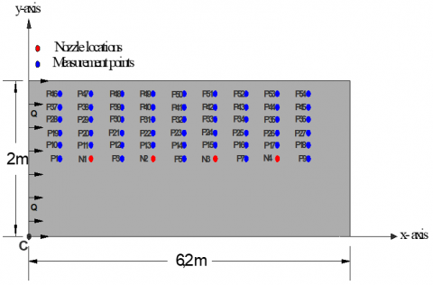
Figure 5. Distribution of measurement points in the model

Measurement points were taken on one side of the model because the flow conditions were symmetrical across the centerline of the model. If we consider point (C) to be the origin point (0,0) for the rest of the points, the coordinates of the measurement points are listed in Table 3.

Velocities near the channel bed were measured by positioning the laser probe adjacent to the sidewall, allowing the laser beam to be guided horizontally toward the measurement zone. This setup made it possible to obtain velocity readings very close to the bed surface. At a few measurement locations, one or two data points near the boundary were excluded from the least-squares analysis, as they were identified as outliers and likely affected by noise in the signal.

To verify the accuracy of the experimental setup and instrumentation, velocity profiles were obtained along the channel centerline at a distance of 4 m from the upstream end. Measurements were conducted under two steady discharges of 10, and 50 m³/hr in the absence of spatially varied (SV), Lateral inflow )nozzle discharge). The experimental conditions associated with these baseline tests are summarized in Table 4.

Table 3. Coordinate of the measurement points

Table 4. Experimental results without SV inflow

Figure 6. Comparison of experimental data with the universal velocity profile

Baseline velocity distributions were first obtained in the absence of spatially varied (SV) inflow in order to provide a reference for identifying the influence of nozzle-induced inflow in subsequent experiments. Figure 6 presents the two velocity profiles measured, expressed in wall coordinates U⁺ and Y⁺. All measurements were conducted with a Manning roughness coefficient of n = 0.016, representing a rough asphalt bed [24, 25]. The Figure also includes the logarithmic velocity distribution equation, which characterizes the inertial sublayer region.

Figure 6 shows that the results of this study are in close agreement with the equation proposed by Nezu and Rodi [26] confirming that both the flume setup and the measurement instruments were properly calibrated and suitable for experiments involving lateral inflow.

Figures 7 to 24 illustrate the distribution of the normalized bed shear stress ($\tau_b$ / $\overline{\tau_{\circ}}$) across the channel width, where $\overline{\tau_{\circ}}$ represents the average shear stress along the wetted perimeter.

Figure 7. Variation of normalized bed shear stress across the model width at x = 0.6 m, and Q = 10 m³/hr

Figure 8. Normalized $\tau_b$ across the model width at x = 1.2 m, and Q = 10 m³/hr

Figure 9. Normalized $\tau_b$ across the model width at x = 1.8 m, and Q = 10 m³/hr

Figure 10. Normalized $\tau_b$ across the model width at x = 2.4 m, and Q = 10 m³/hr

Figure 11. Normalized $\tau_b$ across the model width at x = 3 m, and Q = 10 m³/hr

Figure 12. Normalized $\tau_b$ across the model width at x = 3.6 m, and Q = 10 m³/hr

Figure 13. Normalized $\tau_b$ across the model width at x = 4.2 m, and Q = 10 m³/hr

Figure 14. Normalized $\tau_b$ across the model width at x = 4.8 m, and Q = 10 m³/hr

Figure 15. Normalized $\tau_b$ across the model width at x = 4.8 m, and Q = 10 m³/hr

Figure 16. Normalized $\tau_b$ across the model width at x = 0.6 m, Q = 50 m³/hr

Figure 17. Normalized $\tau_b$ across the model width at x = 1.2 m, Q = 50 m³/hr

Figure 18. Normalized $\tau_b$ across the model width at x = 1.8 m, Q = 50 m³/hr

Figure 19. Normalized $\tau_b$ across the model width at x = 2.4 m, Q = 50 m³/hr

Figure 20. Normalized $\tau_b$ across the model width at x = 3 m, Q = 50 m³/hr

Figure 21. Normalized $\tau_b$ the model width at x = 3.6 m, Q = 50 m³/hr

Figure 22. Normalized $\tau_b$ across the model width at x = 4.2 m, Q = 50 m³/hr

Figure 23. Normalized $\tau_b$ across the model width at x = 4.8 m, Q = 50 m³/hr

Figure 24. Normalized $\tau_b$ across the model width at x = 5.4 m, Q = 50 m³/hr

Figures 7 and 24 demonstrate that at x = 0.6 m and x = 5.4 m, the normalized bed shear stress exhibits only minor transverse variation when compared with the remaining measurement sections. The section at x = 0.6 m lies upstream of the nozzle (N1), at x = 5.4 m corresponds to downstream boundary of the lateral inflow zone. Notably, even with 140% increase in the discharge from each nozzle from q=5 to 12 m³/hr, no discernible influence of lateral inflow on the ($\tau_b$ / $\overline{\tau_{\circ}}$) was detected at measurement locations.

For the remaining cross sections shown in the figures, the ($\tau_b$/$\overline{\tau_{\circ}}$) decreases with increasing streamwise distance (y). At a given cross section, the ($\tau_b$ / $\overline{\tau_{\circ}}$) reaches its maximum at the model centerline and decreases progressively toward the sidewalls. The transverse variation is most pronounced up to approximately half the distance between the model centerline and the model wall. Further downstream, however, this lateral variation becomes less significant, indicating a more uniform distribution of bed shear stress across the model width.

It was observed that the ($\tau_b$/$\overline{\tau_{\circ}}$) does not exhibit significant variation along the model length. A slight increase in normalized bed shear stress may be anticipated in the downstream direction due to the gradual rise in velocity; however, this trend appears to be influenced by the presence of lateral inflow at different measurement sections. A comparison of nozzle discharges (q = 5 and 12 m³/hr) shows that a 140% increase in lateral inflow has not produced a substantial effect on the overall distribution of normalized bed shear stress.

To provide a clearer understanding of bed shear stress behavior, the experimentally measured values between and beneath the nozzle positions are presented in Figures 25 to 36. These results illustrate the spatial variation of shear stresses along the bed in relation to the nozzle inflow.

Figure 25. $\tau_b$ distribution along the model length at y = 1 m, Q = 10 m³/hr, showing the effect of nozzles N1-N4

Figure 26. $\tau_b$ distribution along the model length at y = 1.165 m, Q = 10 m³/hr

Figure 27. $\tau_b$ distribution along the model length at y = 1.33 m, Q = 10 m³/hr

The results indicate that along the model centerline, the measured bed shear stress decreases progressively as the nozzle region is approached. Slightly upstream of the nozzle axis, the stresses become negative, before rising to peak value downstream of the nozzle. A similar pattern is evident for successive downstream nozzles, as shown in Figures 25 and 31. The occurrence of negative bed shear stresses in these regions signifies local flow reversal. This behavior suggests that the nozzle jet impinges on the channel bed and subsequently spreads radially within the surrounding region. At the stagnation point, the bed shear stress reduces to zero.

Figure 28. $\tau_b$ distribution along the model length at y = 1.495 m, Q = 10 m³/hr

Figure 29. $\tau_b$ distribution along the model length at y = 1.66 m, Q = 10 m³/hr

Figure 30. $\tau_b$ distribution along the model length at y = 1.825 m, Q = 10 m³/hr

Figure 31. $\tau_b$ distribution along the model length at y = 1 m, Q = 50 m³/hr

The influence of nozzle discharge on bed shear stress was observed to extend up to y = 1.165 m. This effect intensifies as the nozzle discharge increases from q = 5 to 12 m³/hr. The influence is most evident under low base discharge conditions (Q = 10 m³/hr), as illustrated in Figure 26, and nearly vanishes when the base discharge reaches Q = 50 m³/hr. This behavior is physically consistent: with increasing discharge, both the flow depth and velocity rise, allowing the main flow to overcome the turbulence induced by the nozzle jets, thereby restoring the bed shear stress distribution to its natural state, as depicted in Figure 32.

The interaction between the main model discharge and the nozzle jets causes the inflow to deflect, shifting the impingement region downstream of the jet. This region corresponds to the location where the maximum bed shear stress is observed. Moving laterally away from the nozzle region toward the sidewalls of the model, the variation in bed shear stress decreases. This indicates that the influence of lateral inflow on bed shear stress is strongest directly beneath the nozzle entry points and diminishes at positions farther from the jet.

Figure 32. $\tau_b$ distribution along the model length at y = 1.165 m, Q = 50 m³/hr

Figure 33. $\tau_b$ distribution along the model length at y = 1.33 m, Q = 50 m³/hr

Figure 34. $\tau_b$ distribution along the model length at y = 1.495 m, Q = 50 m³/hr

Figure 35. $\tau_b$ distribution along the model length at y = 1.66 m, Q = 50 m³/hr

Figure 36. $\tau_b$ distribution along the model length at y = 1.825 m, Q = 50 m³/hr

The results show that the $\tau_{\circ_x}$ are strongly affected by the presence of lateral inflow, with the most pronounced variations occurring in the vicinity of the inflow entry points. Along the length of the lateral inflow zone, mean boundary shear stress and mean bed shear stress were evaluated and compared at multiple measurement locations. The findings indicate that mean boundary shear stress increases progressively from the upstream side toward the downstream end of the inflow region. Likewise, the $\overline{\tau_{\mathrm{b}}}$, rises sharply as the flow approaches the lateral inflow zone and continues to increase throughout this region, reaching its highest value at the downstream edge of the inflow zone

The normalized bed shear stress ($\tau_{\mathrm{b}} / \overline{\tau_{\mathrm{o}}}$) exhibits minimal variation at the upstream section (x = 0.6 m) and at the downstream boundary (x = 5.4 m). This indicates that the influence of lateral inflow is negligible at these positions, even with a 140% increase in nozzle discharge.

At intermediate cross-sections, the normalized bed shear stress decreases with increasing streamwise distance. It reaches a maximum at the model centerline and diminishes toward the sidewalls. The transverse variation is significant up to half the distance between the centerline and the wall but becomes less pronounced further downstream, reflecting a more uniform stress distribution across the flume width.

Along the channel length, normalized bed shear stress remains relatively stable. Although a slight downstream increase might be expected due to rising velocity, this effect is weak and strongly influenced by local lateral inflows. Increasing nozzle discharge from q = 5 to 12 m³/hr did not significantly alter the longitudinal distribution of normalized bed shear stress.

Bed shear stress near the nozzles shows a characteristic pattern: it decreases approaching the nozzle, becomes slightly negative upstream of the nozzle axis, and reaches a peak immediately downstream. Negative values indicate local flow reversal caused by jet impingement on the bed, with shear stress reducing to zero at stagnation points.

The impact of nozzle inflow on bed shear stress extends up to y = 1.165 m. This influence is most evident at low base discharges (Q = 10 m³/hr) and nearly disappears at Q = 50 m³/hr. This behavior is physically consistent: higher discharges increase flow depth and velocity, allowing the main flow to suppress nozzle-induced turbulence.

Interaction between the main flow and nozzle jets causes inflow deflection, shifting the impingement zone downstream of the jets where maximum bed shear stress occurs. Moving laterally away from the nozzle region, the influence of lateral inflow weakens, indicating that its effect on bed shear stress is strongest directly beneath the nozzles.

Future research can extend the present findings by investigating the influence of additional hydraulic parameters, such as variable bed roughness, different nozzle orientations, and non-uniform slopes. Incorporating sediment transport into similar experiments would provide further insight into erosion processes associated with spatially varied flow. Numerical simulations using CFD could also complement the experimental dataset by visualizing flow structures. Expanding the full-scale model to other geometries—such as trapezoidal or compound channels—would help generalize the results for broader engineering applications.