M. Premkumar*![]() | S. Rajakumar
| S. Rajakumar![]() | R. Subraja
| R. Subraja![]()
© 2025 The authors. This article is published by IIETA and is licensed under the CC BY 4.0 license (http://creativecommons.org/licenses/by/4.0/).
OPEN ACCESS
This research article pens down to measurement of noise using mathematical expressions for its reduction using digital filter and its information analysis in next generation wireless networks. A noise-corrupted signal in higher frequency ranges is subjected to a digital filter with its characteristics to eliminate the noisy counterpart signal and transmit the signal into a wireless channel in 5G systems. Digital filter design using input-output difference equation is derived and its graphical results from matrix laboratory simulation platform is presented for analysis where research challenges are significant. The recovered information signal is modulated using digital modulation technique of binary phase shift keying (BPSK) and its error rate analysis is depicted. From the simulation results further extension could be done for next generation wireless networks for the upcoming 6G systems.
noise reduction, digital filter, information signal, next generation wireless networks
Measurement is vital in the field of electronics engineering and its applications are essential for developing products globally as that of next generation wireless networks. Developments in the field of next generation wireless networks [1] are marching at a faster pace where information signals are in the form of audio signals, video signals and digital data to cater to various multimedia applications. Audio signal with a bandwidth [2] range of the order of 3 to 3.4 kHz requires optimization in next generation wireless networks and other parameters such as power and data content which are vital for digital data pave a role for next generation wireless networks moving towards millimeter wave concepts [3]. Next generation wireless networks [4] can be projected by mobility models [4] and to assess its metrics for evaluation such as probability of error where the data signal has to be free from noise which is a research challenge, so that information analysis can be done significantly. For such next generation wireless networks, measurement of noise and its reduction for information signal transmission and reception is vital and signal processing techniques such as filtering are needed since an information signal gets corrupted by noise. Filtering of information signal in digital form is done by digital filtering from fundamental prospects such as finite impulse response (FIR) filter or infinite impulse response (IIR) filter based on its impulse response. FIR filters are considered to be more stable and easily designed by window method [5] and IIR filters [6] have a feedback due to the presence of poles. Moreover, IIR filters require only minimal filter coefficients and lesser memory aspects. Further, they are employed for filtering applications irrespective of multimedia signals for processing in present-day 5G systems and forth coming 6G systems.
Noise reduction in speech signal can be done by using Kalman filter [7] which uses concepts of Bayesian state space and prior probability distributions for signal and zero mean Gaussian noise processes. By weighing neighbor pixel locations, a median filter which is distance weighted [8] can reduce noise by estimating local density of noise. Similarly, a Wiener filter [9] having multiple channels can be used for noise reduction and also to enhance the quality of speech signal and also via a median filter for obtaining noise reduced digital images [10]. Noise Reduction of weak current signals by using several methods is presented in the research work which is significant [11]. Also research work [12] proposes a lower complexity recursive algorithm for computing filter weights in a data signal employed in a linear filter and it provides satisfactory performance for noise reduction. Noise corrupted speech signal when subjected to wavelet threshold noise reduction method provides quantitative improvement in terms of error and recovers the speech signal effectively [13]. Filters realized in the form of algorithms such as Kalman filtering algorithms, recursive least squares can be used to reduce noise in displacement sensing signal as proposed in the research [14]. A hybrid filter such as combination of bandpass filter and Wiener filter can reduce noise in a speech signal and provide an improvement in signal to noise ratio (SNR) [15]. Noise reduction performance in terms of mean square error (MSE) is obtained using a Wiener filter [16] and also used for enhancement in speech signal where it is distorted in noise. In the literature [17], a moving average filter provides effective filtering for a noise-affected signal without increasing consumption in power and complexity in contrast to its simple operation standards. In this work measurement of noise and its reduction is done using digital filter with minimal filter coefficients which can contribute to research domain of wireless networks where its information signal analysis is done using binary phase shift keying (BPSK) digital modulation technique.
In order to measure noise and its reduction, considering the scenario in next generation wireless networks where an information carrying signal d(n) experiences a random noise signal w(n) having statistics of Gaussian distribution zero mean and unit variance, the noise corrupted information signal p(n) is given as
$p(n)=d(n)+w(n)$ (1)
where, $d(n)=\cos (2 \pi f n)$, f =0.5pi rad/sec is the digital frequency which is the ratio of the analog frequency fm =1 GHz to the sampling frequency fs=2 GHz for various instants n=0,1,2,…,N-1, and it is further represented as
$p(n)=\cos (2 \pi f n)+w(n)$ (2)
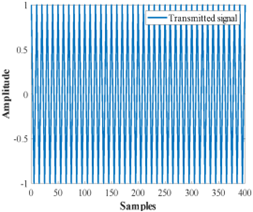
The desired information signal which is transmitted is given in Figure 1, is presented for n comprising of 400 samples and its corresponding amplitude shows the signal of interest.
Figure 1. Transmitted signal
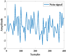
Figure 2. Noise signal
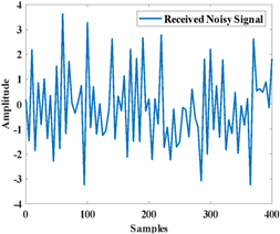
Figure 3. Received noisy signal
The noise signal is graphically represented as in Figure 2, where it is additive white Gaussian noise with mean zero and variance 1 for similar 400 samples.
When a noise signal corrupts an information bearing signal the received noisy signal is shown as in Figure 3.
From the received noisy signal, as given in Figure 3, the information signal needs to be extracted by using a digital filter with its transfer function H(z) needs to be derived. The digital filter considers the noise corrupted signal as its input p(n) and its impulse response is h(n). Correspondingly in the z domain, it is corrupted information signal P(Z), H(Z) and the output signal F(Z). The digital filter can be a resonator filter with poles a1 and a2 resembling that of an infinite impulse response (IIR) filter in the denominator and the numerator N(Z) with a constant M. The input output difference equation for obtaining the filter coefficients is given as
$f(n)+a_1 f(n-1)+a_2 f(n-2)=p(n) M$ (3)
Further the output signal f(n) is
$f(n)=p(n) M-a_1 f(n-1)-a_2 f(n-2)$ (4)
Further proceeding it is given as
$F(Z)=P(Z) M-a_1 z^{-1} F(Z)-a_2 z^{-2} F(Z)$ (5)
$F(Z)+a_1 z^{-1} F(Z)+a_2 z^{-2} F(Z)=P(Z) M$ (6)
$F(Z)\left[1+a_1 z^{-1}+a_7 z^{-2}\right]=P(Z) M$ (7)
$\frac{F(Z)}{P(Z)}=\frac{M}{\left[1+a_1 Z^{-1}+a_2 Z^{-2}\right]}$ (8)
The digital filter for noise reduction is given as
$H(Z)=\frac{F(Z)}{P(Z)}=\frac{M}{\left[1+a_1 Z^{-1}+a_2 Z^{-2}\right]}$ (9)
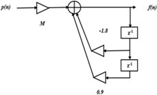
where, a1 and a2 are the filter pole values since it is an infinite impulse response filter (IIR) which has feedback. The values of a1 and a2 need to be determined and they are given as [18] a1=-2Rcosf0 and a2=R2. The pole magnitude of the filter ranges between 0 < R < 1. Similarly the value of gain factor can be found out from $M=(1-R) \sqrt{\left(1-2 R \cos \left(2 f_0\right)+R^2\right.}$. From the above representations, the filter pole values are found to be -1.8831 and 0.9801 based on the calculations for IIR digital filters and the constant M, which is the gain parameter is 0.0061502. Also, on the other hand, if the filter happens to be a finite impulse response (FIR) filter, it has the presence of zeros in the numerator and the noise reduction digital filter transfer function is
$H(Z)=\frac{M\left(1+b_1 z^{-1}+b_2 z^{-2}\right)}{z}$ (10)
with its zeros b1=-2rcosf0 and b2=r2; whereas the value of r is $0 \leq r \leq 1$.
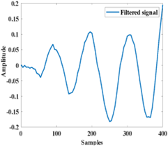
Figure 4. Filtered signal using digital filter
Figure 4 shows the noise-removed signal at the output of the digital filter where the amplitude gradually increases as the number of samples increases. This is due to the presence of poles of the filter which leads to region of convergence in the unit circle so that the digital filter can produce output. The time domain impulse response of the digital filter for the filtered signal [18] can be obtained using partial fraction process and it is:
$h(l)=\frac{M}{\cos f n} R^n \cos (f l+f) u(l)$ (11)
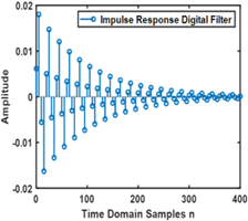
Figure 5. Impulse response of digital filter for noise reduction
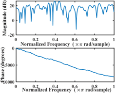
Figure 5 shows the impulse response of the digital filter for noise reduction relating to information for transmission. The time domain filter for observed samples is initially at higher amplitude values and as the number of samples increases, it gradually reduces which can be significant for noise reduction and obtaining the transmitted signal data. Figure 6 shows the frequency response of distorting noise following Gaussian distribution. As the number of samples increases the amplitude values decreases and the noise signal is filtered significantly to obtain the desired information signal. The digital filter can be realized through a structural arrangement as given in Figure 7.
Figure 6. Frequency response and phase response of noise
Figure 7. Digital filter structure for noise reduction structure
The Noise Reduction Ratio (NRR) of the digital filter provides the possible noise reduction which can be achieved by using the noise removal digital filter which is considered and it is measured using the impulse response h(l).
$N R R=\frac{\sigma_f^2}{\sigma_p^2}=\sum_{l=0}^{\infty} h_l^2$ (12)
Using the value of R, and the considered pole values, gain as per (9), the NRR value can be found on expansion of (12).
$N R R=h_1^2+h_2^2+h_3^2+h_4^2+\cdots+h_{399}^2$ (13)
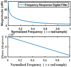
Figure 8. Frequency response and phase response of noise reduction filter
Substituting the values of impulse response coefficients obtained from the digital filter the NRR value as per MATLAB simulation reaches 0.02. Whenever NRR [18] value is less than one, input noise gets attenuated by the considered digital filter.
Figure 8 shows the frequency response in radians/sample for the considered digital filter and its phase values in degrees. For the designed frequency of 1GHz expressed in radians per sample and the phase value in degrees it is also represented for the digital filter which is taken into consideration for noise reduction.
The filtered information signal is mapped using a digital modulation scheme depending on the positive and negative amplitude values obtained after noise removal. A noise-corrupted signal is recovered through a digital filter and it is further detected when it passed through a wireless channel. It can be detected at the receiver in next generation wireless networks. The next generation wireless system can be mathematically represented as
$r_{\text {filtered }}(l)=d_s(l) h_{\text {fad }}(l)+v(l)$ (14)
where, $d_s(l)$ is the binary phase shift keying (BPSK) digital modulation scheme which transmits binary 1s and 0s using phase shifts of 0 and 180 degrees where each digital data signal is a symbol for transmission and detection. BPSK uses only a single bit for a symbol so as the data rate also depends on the considered bit symbol. Further variants of BPSK such as 4-PSK which is also quadrature phase shift keying (QPSK) which has two bits per symbol with four different phase values. The recovered digital signal filter positive values are mapped to +1 and negative values of the digital signal filter are mapped to -1. As per BPSK scheme of digital modulation +1 represents binary 1 and -1 represents binary 0 which forms a possibility to map the filtered data as digital data for transmission in next generation wireless network at the baseband level.
Also, the fading channel represented as $h_{f a d}(l)$ is the fading channel coefficients experiencing flat fading or frequency selective fading and $v(l)$ is the receiver noise following Gaussian distribution. Flat fading channel has lesser signal bandwidth and large channel bandwidth, whereas frequency selective fading channel is its vice versa.
The flat fading channel following Rayleigh distribution can be given as
$h_{f a d}(l)=\propto_{f a d}(l) \exp ^{i \emptyset(l)}$ (15)
The probability density function (PDF) for the channel condition $h_{f a d}$ considering a particular time instant, the noise removed signal with digital data is
$p\left(h_{f a d}\right)=\frac{h_{f a d}}{\sigma^2} e^{-\frac{h_{f a d^2}}{2 \sigma^2}}$ (16)
The probability density function (PDF) of receiver noise follows Gaussian distribution given by
$v(l)=\frac{1}{\sqrt{2 \pi \sigma_l^2}} \exp ^{-\left(\frac{\left(l-\mu_l\right)^2}{\sigma_l^2}\right)}$ (17)
where mean $\mu_l$ and variance $\sigma_l^2$. For a complex valued signal, the variance is given as the noise power where the real part is 0.5 and the imaginary part is 0.5 so that noise power/variance reaches towards unity where it resembles an additive white Gaussian noise (AWGN) channel. Similarly, for frequency selective fading channel obtained using a power delay profile (PDP) which has a signal bandwidth greater than the channel bandwidth, the channel impulse response is
$\begin{gathered}h_{f a d}(l ; \tau)= \sum_{k=0}^{N-1} \alpha_{f a d k}(l, \tau) \exp ^{i 2 \pi f \tau_k \emptyset(l, \tau)} \delta\left(\tau-\tau_k(l)\right)\end{gathered}$ (18)
Further, flat fading time varying channel has signal duration to change for a particular time instant depending on the speed of which the transmission signal changes with doppler shift for a particular velocity. The doppler shift is considered to be relative movement between the transmission terminal and the reception terminal which can be a mobile terminal or a base-station representing signals for uplink and downlink conditions. A shift in frequency gets added with the carrier frequency when positive doppler is observed and gets reduced when the doppler is negative. Based on this detection metric the next generation wireless network can be assessed for its probability of error. The probability of error of next generation wireless network is given by graphical analysis after measurement of noise and its reduction through the digital filter. Table 1 gives the considered parameters for simulation in matrix laboratory.
Table 1. Simulation data and its simulation values
|
Simulation Data |
Simulation Values |
|
Analog Signal |
1 GigaHertz(GHz) |
|
Sampling Signal |
2 GigaHertz(GHz) |
|
Digital Frequency |
0.5pi rad/sec |
|
Noise Reduction Filter |
Digital IIR filter |
|
Fading Channel |
AWGN channel, Flat fading, Frequency Selective Fading, Time Varying Channel |
|
Signal to Noise Ratio |
0 to 30 dB |
|
Probability of Error |
10-1 to 10-3 |
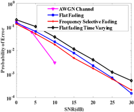
Figure 9. Probability of error analysis against signal to noise ratio
Figure 9 graphically demonstrates the filtered signal probability of error in various multipath fading channels. The additive white Gaussian noise channel is not a physical channel and it only represents the noise due to movement of electrons in the receiver. To obtain a probability of error of 10-2 flat fading channel takes 13 dB, whereas a frequency selective fading channel specified by a power delay profile takes 12 dB and time varying channel takes beyond 15 dB for each and every time instant. This is because of the time varying nature of the channel which is highly degrading due to changes in symbol parameters based on the impulse response of the channel coefficients.
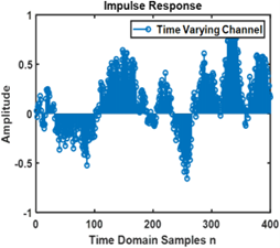
Figure 10. Impulse response of time time-varying channel
Figure 10 shows the impulse response of the time-varying channel with a velocity of 10 km/hr observed for 400 samples. This sort of channel categorizes itself in fast fading statistics in which the impulse response coefficients changes in a particular data signal duration for a symbol possibly comprising of single bit in respect of BPSK. However, the channel conditions will also tend to change when the doppler shift changes with respect to velocity in which the transmitter terminal exhibits mobility in comparison the receiver terminal probably a base station in next generation wireless network. Hence information signal detection needs data denoising [19] or noise suppression [20] which can contribute towards noise reduction, from a data signal perspective for wireless networks.
This research work concludes with analysis that noise can be measured graphically for various samples and can be eliminated to significant extent where it is used for signal transmission and reception in next generation wireless communication systems. The designed digital IIR filter can provide stable response depending on the poles selection within the range of operation. Measurable noise as well as noise removed signals can be employed for upcoming electronic systems where many products are being introduced for societal applications relevant to next generation wireless networks for intended 6G systems. As a future work more research findings can be explored for next generation wireless networks taking into consideration of noise reduction techniques employed at a system level.
[1] Shafl, M., Aamer, W., Butterworth, K. (2001). Next generation wireless networks. In 2001 IEEE International Symposium on Circuits and Systems (ISCAS), Sydney, NSW, Australia, pp. 7.2.1-7.2.9. https://doi.org/10.1109/TUTCAS.2001.946969
[2] Shakhov, V., Koo, J., Choo, H. (2006). Bandwidth optimization in next generation wireless network. In COIN-NGNCON 2006 - The Joint International Conference on Optical Internet and Next Generation Network, Jeju, Korea (South), pp. 150-152. https://doi.org/10.1109/COINNGNCON.2006.4454593
[3] Foty, D. (2007). Next-generation wireless networks: A new world, from bottom to top. In AFRICON 2007, Windhoek, South Africa, pp. 1-9. https://doi.org/10.1109/AFRCON.2007.4401584
[4] Santi, P. (2012). Next generation wireless networks. In Mobility Models for Next Generation Wireless Networks: Ad Hoc, Vehicular and Mesh Networks. https://doi.org/10.1002/9781118344774.ch1
[5] Eleti, A.A., Zerek, A.R. (2013). FIR digital filter design by using windows method with MATLAB. In 14th International Conference on Sciences and Techniques of Automatic Control & Computer Engineering - STA'2013, Sousse, Tunisia, pp. 282-287. https://doi.org/10.1109/STA.2013.6783144
[6] Shakibaei, B.H., Shawon, M.J., Gang, S.Y., Adikan, F.R.M. (2014). IIR filter implementation of dispersive medium using Z-transform. In 2014 IEEE 5th International Conference on Photonics (ICP), Kuala Lumpur, Malaysia, pp. 211-213. https://doi.org/10.1109/ICP.2014.7002358
[7] Sarafnia, A., Ghorshi, S. (2013). Noise reduction of speech signal using Bayesian state-space Kalman filter. In 2013 19th Asia-Pacific Conference on Communications (APCC), Denpasar, Indonesia, pp. 545-549. https://doi.org/10.1109/APCC.2013.6766008
[8] Baek, S., Jeong, S., Choi, J.S., Lee, S. (2015). Impulse noise reduction using distance weighted average filter. In 2015 21st Korea-Japan Joint Workshop on Frontiers of Computer Vision (FCV), Mokpo, Korea (South), pp. 1-5. https://doi.org/10.1109/FCV.2015.7103733
[9] Shamsa, A., Ghorshi, S., Joorabchi, M. (2016). Noise reduction using multi-channel FIR warped Wiener filter. In 2016 13th International Multi-Conference on Systems, Signals & Devices (SSD), Leipzig, Germany, pp. 531-536. https://doi.org/10.1109/SSD.2016.7473687
[10] Mikolajczak, G., Peksinski, J. (2016). Estimation of the variance of noise in digital images using a median filter. In 2016 39th International Conference on Telecommunications and Signal Processing (TSP), Vienna, Austria, pp. 489-492. https://doi.org/10.1109/TSP.2016.7760927
[11] Jiao, Z., Lixiang, J., Huang, J., Sun, J., Juan, N., Wang, J. (2018). Analyses on methods for noise reduction of weak current signals. In 2018 Eighth International Conference on Instrumentation & Measurement, Computer, Communication and Control (IMCCC), Harbin, China, pp. 641-644. https://doi.org/10.1109/IMCCC.2018.00139
[12] Zhao, Y., Chen, J., Chen, J. (2019). Recursive variable span linear filter for noise reduction. IEEE Signal Processing Letters, 26(12): 1902-1906. https://doi.org/10.1109/LSP.2019.2953817
[13] Zhang, N., Wang, Z. (2020). Noise reduction of speech signal based on wavelet transform with improved threshold function. In 2020 12th International Conference on Measuring Technology and Mechatronics Automation (ICMTMA), Phuket, Thailand, pp. 542-547. https://doi.org/10.1109/ICMTMA50254.2020.00122
[14] Li, C., Huang, R., Yi, Y., Bermak, A. (2020). Investigation of filtering algorithm for noise reduction in displacement sensing signal. IEEE Sensors Journal, 21(6): 7808-7812. 10.1109/JSEN.2020.3048511
[15] Liu, R. (2022). Speech noise reduction system based on combined filter. In 2022 IEEE Conference on Telecommunications, Optics and Computer Science (TOCS), Dalian, China, pp. 611-616. https://doi.org/10.1109/TOCS56154.2022.10016136
[16] Nuha, H.H., Absa, A.A. (2022). Noise reduction and speech enhancement using wiener filter. In 2022 International Conference on Data Science and Its Applications (ICoDSA), Bandung, Indonesia, pp. 177-180. https://doi.org/10.1109/ICoDSA55874.2022.9862912
[17] Panetas-Felouris, O., Pagkalos, K. P., Vlassis, S. (2024). Moving average filter in time-mode signal processing. In 2024 Panhellenic Conference on Electronics & Telecommunications (PACET), Thessaloniki, Greece, pp. 1-4. https://doi.org/10.1109/PACET60398.2024.10497041
[18] Orfanidis, S.J. (1995). Introduction to Signal Processing. Prentice-Hall, Inc.
[19] Letafati, M., Ali, S., Latva-Aho, M. (2024). Conditional denoising diffusion probabilistic models for data reconstruction enhancement in wireless communications. IEEE Transactions on Machine Learning in Communications and Networking, 3: 133-146. https://doi.org/10.1109/TMLCN.2024.3522872
[20] Feng, Z. (2024). Complex noise suppression using a robust dictionary learning approach. IEEE Geoscience and Remote Sensing Letters, 22: 7502405. https://doi.org/10.1109/LGRS.2024.3514077