Ahmed Rifaat Hamad![]() | Aqeel N. Abdulateef
| Aqeel N. Abdulateef![]() | Bayan Mahdi Sabbar
| Bayan Mahdi Sabbar![]() | Mohannad Jabbar Mnati*
| Mohannad Jabbar Mnati*![]() | Adnan Hussein Ali
| Adnan Hussein Ali![]() | Alex Van Den Bossche
| Alex Van Den Bossche![]()
© 2025 The authors. This article is published by IIETA and is licensed under the CC BY 4.0 license (http://creativecommons.org/licenses/by/4.0/).
OPEN ACCESS
In recent years, the role of the Internet of Things (IoT) in monitoring and predicting various environmental phenomena has expanded significantly. This study presents the design and implementation of an intelligent IoT ecosystem tailored for weather monitoring stations. The core objective of this system is to enhance the accuracy and responsiveness of weather forecasting by integrating machine learning (ML) techniques. This scalable IoT ecosystem efficiently collects comprehensive meteorological data from all sensors, such as temperature, humidity, and atmospheric pressure, using an ESP32 as a microcontroller. This combination of specialized hardware and advanced software techniques markedly boosts prediction accuracy, presenting a pioneering step in environmental monitoring methodologies. These algorithms are well-known for their adaptive learning capabilities and dynamically update predictions based on real-time and historical datasets. With the strategic inclusion of cloud computing, data accessibility and scalability have been remarkably enhanced. This amalgamation of specialized hardware, intelligent software, and cloud infrastructure significantly amplifies prediction accuracy, heralding a new era in environmental monitoring methodologies.
IoT, ML, ESP32, temperature sensor, humidity sensor, pressure sensor, weather station
Atmospheric observations were made by ancient people using simple equipment like wind vans and water clocks. During the 17th and 18th centuries, barometers were introduced alongside thermometers and hygrometers which gave better readings than before. The late 20th century witnessed the development of automated weather stations. These stations can record data autonomously, reduce human errors, and enable continuous monitoring.
Weather forecasting has evolved significantly over the past century. Traditional methods relied on manual observations, empirical rules, and basic statistical models. In the mid-20th century, the introduction of numerical weather prediction (NWP) models marked a major leap, utilizing early computers to solve mathematical equations that simulate atmospheric behavior. These models, though groundbreaking, were limited by computational capacity and data availability.
By the late 20th and early 21st centuries, advancements in satellite technology and remote sensing dramatically improved the accuracy and resolution of meteorological data. However, despite these improvements, challenges remained in forecasting localized and rapidly changing weather patterns.
The IoT began to influence the IT scene at the beginning of the twenty-first century. Sensors are cheaper, more compact, and networked. To provide more extensive data collection and remote data access, weather stations have begun integrating these sensors.
The amount of data increased with data collection capacity. As a solution, cloud-computing systems with scalable processing and storage capacities have been developed. Big meteorological data began during this period, when large datasets were accessible for study [1-5].
Although statistical techniques have long been employed in weather forecasting, machine learning research has been spurred by the availability of large datasets. It is now possible to train algorithms on past data to identify anomalies and make more accurate predictions.
The potential for combining the Internet of Things (IoT) and machine learning became apparent at a pivotal point in the mid-2010s. This means that in weather monitoring, real-time actionable insights must be derived in addition to data collection. This made short-term hyper-local forecasts, real-time anomaly detection, and feasible predictive equipment maintenance.
Today, a number of cutting-edge technologies have come together in the design and execution of weather monitoring systems. Currently, IoT sensors can gather a wide variety of data from UV radiation to soil moisture. These data were analyzed using machine learning models, which provide predictions with previously unknown accuracy. These models include neural networks, decision trees, and algorithms such as Naive Bayes. These integrated systems are essential tools for many industries, from urban planning to agriculture, as they offer decision-making insights in addition to data.
Based on Bayes' theorem, the Naive Bayes algorithm has been applied in several fields, including meteorology, as in our study. Using past data and other atmospheric indications, a weather station can use this supervised machine-learning technique to forecast weather conditions, such as rain, sunshine, or snow. By training a Naive Bayes classifier with inputs, such as humidity, temperature, and barometric pressure, one can learn to identify patterns in the data and forecast the probability of a certain weather event. In spite of its 'naive' assumption of feature independence, this algorithm frequently yields remarkably accurate results, which makes it an economical and useful tool for short-term weather forecasting [6-11].
The purpose of this study is to design and implement an intelligent IoT and machine-learning-based weather monitoring station system. Weather station monitoring involves the collection of atmospheric data to predict, understand, and analyze weather patterns. With the advent of the Internet of Things (IoT), it has become easier to create DIY weather stations and monitor them remotely in real time [12, 13].
The block diagram of the proposed system is represented in Figure 1. A weather monitoring IoT system consists not only of an array of sensors for collecting the environmental data but also a microcontroller that processes the sensor output and communicates the results. The paper employs several sensors and hardware components to monitor the ambient conditions that influence varying degrees of macro weather, quantifying air pressure, temperature, and humidity. The BMP180 sensor is for air pressure, and the DHT11 sensor is for temperature and humidity measurement. This provides a real-time reading on the environment, meaning that no access to the data via the cloud is necessary (by using an I2C LCD2004 module). The ESP32 and sensors power supply go through a breadboard DC power supply to make the voltage distribution stable.
The system employs cloud computing for the storage, access, and real-time scaling of data using ThingSpeak. Sensor data from the ESP32 is sent to ThingSpeak, which offers comprehensive capabilities for querying and visualizing past data for feedforward machine learning models. It is scalable, enabling the processing of data from several weather monitoring stations, hence facilitating remote monitoring and analysis. This smartphone app displays real-time weather data from ThingSpeak, and users can check out historical trends and future predictions. This enhances the overall user experience by making it easier for users to get predictions and data anywhere, at any time.
Figure 1. The block diagram of the proposed system
This section presents the design of the system in addition to showcasing related work in the same field. These works include similar studies that use different technologies and approaches, such as those that use different types of sensors for weather stations, microcontrollers, wireless communication technologies, and monitoring devices.
The weather station designed in this study consists of temperature, humidity, and air pressure sensors; an ESP32 microcontroller; Wi-Fi as a wireless communication system; ThingSpeak Cloud for storage and monitoring data; and a new Android app for smartphones that is intended to track the measured data from the weather station. The devices utilized in prior projects in this field are listed in Table 1.
Table 1. The list of related work papers
|
Related Work |
Type of Sensors |
Type of Microcontroller |
Type of Communication |
IoT |
Monitoring |
Cloud |
|
Mabrouki et al. [1], 2021 |
DHT22, Ozone, Nitrogen dioxide, Sulfur dioxide |
Arduino UNO |
Wi-Fi |
NO |
Terminal |
NO |
|
Djordjevic and Dankovic [2], 2019 |
BME280, MQ-2, BH1750 |
PIC18F45K22 |
GSM |
YES |
LCD 1602 |
YES |
|
Bella et al. [5], 2023 |
DHT11, Rain Sensor, Bmp 180 |
ESP8266, |
Wi-Fi |
YES |
Terminal |
YES |
|
Kim et al. [14], 2018 |
SHT-21, Rain Sensor, Wind speed, wind direction |
Arduino |
GSM |
YES |
Terminal |
YES |
|
Nallakaruppan and Kumaran [15], 2019 |
DHT-11, BMP-180, Rainfall Sensor |
Raspberry Pi 3 |
Wi-Fi |
NO |
LCD 1602 |
NO |
|
Shahadat et al. [16], 2020 |
DHT11, BMP-180, Rain Sensor |
ESP8266 |
Wi-Fi |
YES |
Terminal |
YES |
|
NarasimhaRao et al. [17], 2020 |
SHT10, DHT 11, MG 811, TSL251 |
Arduino UNO and ESP8266 |
Wi-Fi |
YES |
Terminal |
YES |
The Intelligent IoT Ecosystem for Weather Monitoring seamlessly blends advanced IoT sensors and machine-learning algorithms to revolutionize meteorological data capture and interpretation. Strategically positioned sensors gather essential weather metrics and transmit them via advanced wireless protocols to a centralized data repository. These raw data are then processed by machine learning models to detect patterns and forecast weather changes. Insights are readily accessible to users through an intuitive interface, whereas a feedback loop ensures continuous system refinement and increased accuracy over time.
3.1 Hardware components
In this part, every electronic component utilized in this project will be presented.
3.1.1 ESP32 Microcontroller
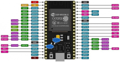
The ESP32 shown in Figure 2 is a versatile and powerful microcontroller developed by Espress. This is particularly noteworthy for its integration of both Wi-Fi and Bluetooth (classic and BLE) capabilities within a single chip. Building on the success of its predecessor, ESP8266 (primarily known for Wi-Fi), ESP32 provides a more comprehensive set of features, including a more extensive GPIO count, enhanced processing power with its dual-core Ten silica LX6 microprocessor, and better power management.
Figure 2. Pin diagram of Node MCU ESP32 [18]
Developers appreciate the ESP32 for its compatibility with various development environments, including the popular Arduino IDE and the advanced ESP-IDF. The main properties of Node MCU ESP32 are listed in Table 2 [18].
Table 2. Main properties of NODEMCU ESP32 [18]
|
Property |
Details |
|
Processor |
Dual-core Tensilica LX6 microprocessor |
|
Clock Frequency |
Up to 240 MHz |
|
RAM |
~520 KB Internal SRAM |
|
Flash Memory |
External, varies (commonly 4 MB) |
|
Wi-Fi |
802.11 b/g/n (2.4 GHz) |
|
Bluetooth |
Classic + BLE (Bluetooth Low Energy) |
|
GPIO Pins |
Typically up to 36 pins |
|
ADC |
Up to 18 channels (12-bit) |
|
DAC |
2 channels (8-bit) |
|
UART, I2C, SPI |
Multiple channels/interfaces |
|
Temperature Sensor |
Internal |
BMP180 in Figure 3 is a popular sensor for measuring temperature and barometric pressure. Atmospheric pressure varies with both weather and altitude, and both can be measured using this sensor. Manufactured by Bosch Sensor Tec, it has been widely used in various applications ranging from weather stations to altitude estimations. Table 3 lists some key properties and features [19].
Figure 3. BMP180 sensor module [19]
Table 3. Main properties of BMP180 sensor [19]
|
Property |
Details |
|
Supply Voltage |
1.8V to 3.6V |
|
Interface |
I²C (100kHz and 400kHz speeds) |
|
Pressure Range |
300 hPa to 1100 hPa (+9000m to -500m) |
|
Pressure Resolution |
Adjustable: 0.06 hPa to 0.02 hPa |
|
Pressure Accuracy |
Absolute: ±1 hPa |
|
Power Consumption |
3µA during pressure measurement |
|
Temperature Range |
-40°C to +85℃ |
|
Temperature Resolution |
0.1℃ |
|
Temperature Accuracy |
Absolute: ±1℃ |
3.1.3 DHT11 sensor
A simple, very affordable digital temperature and humidity sensor is the DHT11, shown in Figure 4. It detects the air quality around it using a thermistor and a capacitive humidity sensor, then outputs a digital signal on the data pin. It's not too difficult to use. Table 4 displays the primary characteristics of the DHT11 sensor module [20].
Figure 4. DHT11 sensor module [20]
Table 4. The main properties of DHT11 sensor [20]
|
Property |
Details |
|
Supply Voltage |
3.3V to 5V |
|
Humidity Range |
20% to 90% RH |
|
Humidity Resolution |
1% RH |
|
Humidity Accuracy |
±5% RH |
|
Temperature Range |
0°C to 50℃ |
|
Temperature Resolution |
1℃ |
|
Temperature Accuracy |
±2℃ |
|
Response Time |
Approximately 1 second |
|
Power Consumption |
0.5mA (measurement), 100µA |
There are three phases in the communication process: sending a request to the DHT11 sensor, waiting for a return pulse from the sensor, and then beginning the data transmission to the microcontroller. The single-bus data format utilized for synchronization and communication between the MCU and DHT11 sensor is depicted in Figure 5a. An approximate 4 ms communication procedure occurs. Decimal and integral components make up data. The sensor transmits higher data bits first, with a 40bit total data transmission. The MCU is seen in Figure 5b, transmitting the start signal and receiving DHT answers [20].
(a)
(b)
Figure 5. a) DHT11 Sensor communication process, and b) MCU sending out the start signal and DHT responses [20]
3.1.4 I2C LCD2004 module
The LCD2004 module in Figure 6 is a user-friendly 20 × 4 liquid crystal display that leverages the I2C communication protocol, allowing for efficient interfacing with microcontrollers using only two data lines: SDA and SCL. By simplifying traditional LCD connections, this module reduces pin usage, making it ideal for projects with limited GPIO availability [21].
Figure 6. I2C LCD2004 module [21]
3.1.5 Breadboard DC power supply
Figure 7 displays the breadboard power supply and Table 5 lists the breadboard's primary characteristics. Its two channels provide configurable output between 3.3V and 5V. The maximum amount of current that can be drawn is 700 mA. The user may choose the output voltage by adjusting the jumpers individually, and this decision is independent of the channel.
Figure 7. DC power supply module [22]
A breadboard power supply is a compact and convenient module designed to provide regulated voltage directly to a solderless breadboard, which is commonly used in electronic prototyping. These power supplies are designed to fit onto the breadboard and provide selectable voltage levels, often 3.3V and 5V, which are standard voltages for many electronic components and microcontrollers [22].
Table 5. The main properties of DC power supply [22]
|
Property |
Details |
|
Input Voltage |
Often 6.5V to 12V (from a DC adapter) |
|
Output Voltage Options |
Commonly 3.3V and 5V (selectable) |
|
Maximum Current |
Varies (common values include 500mA or 700mA) |
|
Voltage Regulation |
Linear regulator (like LM317) or switching regulator (like LM2596) |
|
On/Off Switch |
Typically included |
|
Indicator LEDs |
Often present to show power status |
|
Protection Features |
Overcurrent, short-circuit, sometimes thermal |
3.2 Software requirements
3.2.1 Arduino IDE software
The Arduino IDE is an open-source software environment. was used to create and upload code to boards that were compatible with Arduino. It offers extensive functionality for seasoned developers while being user friendly. As an essential tool in the Arduino ecosystem for prototyping and electronics exploration, the IDE supports a range of Arduino boards and offers an easy method to add libraries and examine sample projects. The main window of the IDE is shown in Figure 8 [23].
Figure 8. Main Arduino IDE platform widow [23]
3.2.2 ThingSpeak cloud
MathWorks created ThingSpeak, an IoT analytics platform that provides cloud-based data aggregation, visualization, and analysis. ThingSpeak facilitates the gathering, storing, and understanding of real-time data by seamlessly integrating with connected devices. Its compatibility with MATLAB makes complex data processing and analytics possible. ThingSpeak is an adaptable option for IoT data management, supporting applications ranging from simple hobby projects to intricate industrial monitoring systems, all with a focus on real-time data display. Figure 9 shows the main webpage window of the ThingSpeak cloud [24].
Figure 9. The website window of ThingSpeak cloud [24]
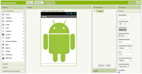
3.2.3 MIT App inventor
Figure 10 shows the MIT APP Inventor main webpage window. MIT created an open-source web-based platform called MIT App Inventor to make the process of creating Android apps easier. Even those without any previous coding experience may design functioning mobile apps with intuitive drag-and-drop interfaces. With the App Inventor, a platform for quick prototyping and teaching, a wide variety of individuals can now easily convert their ideas into functional mobile applications [25].
Figure 10. Website window of MIT App Inventor [25]
3.3 Machine learning integration
Under artificial intelligence lies machine learning, which allows self-learning from data through zero explicit programming requirements, enabling its integration into different systems in different domains, enhanced system functionality, automation of complex operations, and predictive capabilities [15]. The Naïve Bayes classifier is one of the fundamental algorithms within machine learning.
Naive Bayes is a probabilistic machine learning algorithm that can be used in various classification tasks based on Bayes’ theorem. It operates based on the principle of independence among predictors. Simplicity and efficiency are some features distinctively associated with this type of naive Bayesian classifier [16]. Institutions may benefit from incorporating such models into their frameworks since they expose new dimensions for analysis that were previously difficult or not possible at all [17]. To prevent any knowledge gaps, we will cover in detail the Naïve Bayes method and related topics in this chapter [26, 27]. Bayes’ theorem is a simple mathematical procedure for calculating conditional probabilities. Conditional probability is the probability of an event occurring given that another event has (assuming, supposing, stating, or asserting) occurred, as in Eq. (1).
$P(A \mid \mathrm{B})=(P(B \mid \mathrm{A}) P(A)) /(P(B))$ (1)
where:
P(A|B): how often does A happen given that B happens? (Is called posterior probability)
P(B|A): how often does B happen given that A happens?
P(A): how likely A is on its own?
P(B): how likely B is on its own?
By using the chain rule, the likelihood P(A|B) can be decomposed, as shown in Eq. (2):
$\begin{gathered}P(A \mid B)=P\left(A_1, A_2, \ldots \ldots, A_n \mid B\right)= \\ P\left(A_1 \mid A_2, \ldots A_n, B\right) * P\left(x_2 \mid x_3, \ldots x_n, B\right) P\left(A_n \mid B\right)\end{gathered}$ (2)
However, the conditional probabilities are independent of each other because of the naive conditional independence principle (As in Eq. (3)).
$P(A \mid B)=P\left(A_1 \mid B\right) * P\left(A_2 \mid B\right) P\left(A_n \mid B\right)$ (3)
As a result, conditional independence gives us results in Eq. (4).
$\begin{gathered}P(B \mid \mathrm{A})=\left(P\left(A_1 \mid B\right) * P\left(A_2 \mid B\right) P\left(A_n \mid B\right) *\right. \\ P(B)) /\left(P\left(A_1\right) * P\left(A_2\right) P\left(A_n\right)\right)\end{gathered}$ (4)
Furthermore, because the denominator is constant across all values, the posterior probability may be as in Eq. (5)
$P\left(A_1, A_2, \ldots \ldots, A_n \mid B\right) \alpha P(B) \prod_{i=1}^n P\left(A_1 \mid B\right)$ (5)
The Naive Bayes classifier uses this model in conjunction with a decision rule. Selecting the hypothesis with the greatest probability is a commonly used guideline known as the maximum a posteriori (MAP) decision rule, as shown in Eq. (6).
$B=\operatorname{argmax}_B P(B) \prod_{i=1}^n P\left(A_1 \mid B\right)$ (6)
The process of using the Naive Bayes algorithm to process environmental parameters (such as temperature, humidity, pressure, and altitude) on an ESP32 starts with the collection of an adequate dataset. This dataset was collected manually in Iraq with relevant sensors attached to an ESP32 microcontroller. For accurate environment readings, sensors such as DHT22 (Temperature and humidity) and BME280 (Pressure and Altitude) were utilized. These data were collected and logged periodically and saved into a structured file such as CSV, where each line contained data of the readings from each sensor in addition to a label, either "normal" or "alert" depending on whether the environment was as expected. This is the base data we use to train a machine learning model.
After the dataset was obtained, we leveraged Python using the scikit-learn library to train a Naive Bayes classification model. Using the panda’s library, the data were imported into a Python script and split into input features (temperature, humidity, pressure, and altitude) and output labels. The data were subsequently separated into training and testing subsets through the conventional 80/20 split. The model was trained on the training set and tested on the validation set using a Gaussian Naive Bayes approach. The accuracy of the model was determined, and the reliability of the model to predict environmental settings based on new sensor data was established.
Following training, the model was used to extract its internal parameters called mean and variance for each feature across each class, as well as the class prior probabilities. These parameters are critical for running the Naive Bayes decision-making logic directly on the ESP32. A header file named "model. These two angles were generated, as constants or arrays in C/C++ format, by the h, which means "header. This file is included in the Arduino IDE project, allowing the ESP32 to do real-time classification with the Naive Bayes algorithm. This means using ML, the ESP32 can process the sensor data and classify environmental conditions as normal or alert without assistance from a server or cloud-based ML service.
The ESP32 microcontroller and weather station sensors were integrated to create the final device used in this project after they were thoroughly explained in the preceding section, which also covered all electronic elements and software used in the programming. Figure 11 shows the completed block diagram architectural circuit created using the Fritzing electrical and electronic circuit design applications.
Fritzing is an open-source initiative aimed at supporting designers, artists, researchers, and hobbyists in working creatively with interactive electronics. It provides a software application that allows users to record and share their prototypes, educate them on electronics in a classroom, and design PCB layouts for commercial manufacturing. Beginners may more easily comprehend and design electronics owing to Fritzing's user-friendly interface, which makes it possible to create electronic circuits via visual representations [28].
Figure 11. Monitoring system's block diagram architecture
After the Naive Bayes algorithm, which is a probabilistic classification technique based on Bayes' theory, was used in our research and applied to weather forecasting, it can now be used to predict weather conditions based on historical weather data. By training on past weather patterns and associated conditions, a Naive Bayes classifier can determine the probability of a specific weather outcome occurring, given a new set of input data from the sensors in real-time.
The Naive Bayes algorithm was used in this study only to generate data for fore-casting weather that will be used and relied upon in programming the final practical circuit. The programming focused on temperature and humidity, given that the place where the measurement was made is the same in terms of atmospheric pressure; therefore, it does not affect the results in the programming.
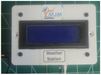
The primary function of this system is to monitor meteorological parameters such as air pressure, temperature, and humidity, and utilize the results to anticipate the weather. As shown in Figure 12, the smart weather station prototype was implemented in a laboratory setting. BMP180 and DHTT sensors, together with an ESP32 microcontroller, were used to create the prototype.
Figure 12. The monitoring hardware system's architecture
The complete system was programmed using three different programs: one for measuring and sending circuit results, another for cloud monitoring via ThingSpeak, and a third for smartphone applications. Figure 13 shows a flowchart of the measurement circuit. The flowchart illustrates how the ESP32 measures gathered and presented data from the sensors (temperature, humidity, and air pressure) on the LCD screen. If Wi-Fi is accessible, the data are transferred and uploaded to the cloud.
Figure 13. The flowchart of the weather station system
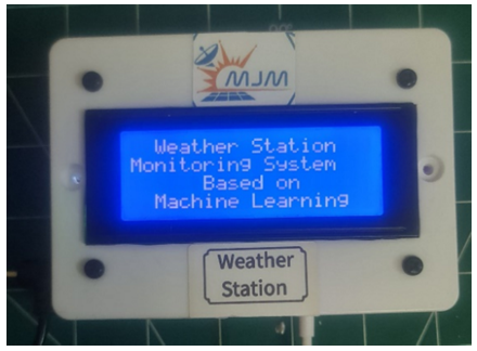
Figure 14 (a) shows the monitoring system at the start of the operation, as well as taking one of the readings after it is turned on. Figure 14 (b) shows the readings (temperature, humidity, altitude, and air pressure), and the result or confirmation of the Naive Bayes algorithm can be observed in the first row of the LCD.
(a)
(b)
Figure 14. The monitoring circuit with deferments results
ThingSpeak is often used for IoT system proof-of-concept and prototypes that require analytics. The cloud-based IoT analytics platform ThingSpeak was used to evaluate the condition of the completed system and display the real-time data streams. Figure 15 shows the findings of this study. ThingSpeak displays data in real-time that it gets from a weather station gadget. A specialized software created for this purpose will display the same findings on smartphones when all data and results have been submitted to the ThingSpeak website, as shown in Figure 16.
Figure 15. ThingSpeak website window with results (temperature, humidity, air pressure, and altitude)
Figure 16. Smart phone window with system results (temperature, humidity, air pressure, and altitude)
These IoT systems, like the ESP32-based environmental monitors, provide huge benefits through the real-time data they gather, making resource management and sustainability easier than ever. But on freshening it up with their scale, they can contribute to electronic waste, the pollution that comes from battery usage, and energy consumption. Energy-efficient designs, sustainable materials, and proper recycling practices should be used to minimize their impact on the environment.
As the proposed ESP32-based environmental monitoring system is an example of an Internet of Things (IoT) system, running in potentially energy-constrained environments, the need for power management to facilitate long-lived, reliable deployments becomes a primary concern. ESP32 microcontroller is very powerful, but it also consumes a lot of energy when working Wi-Fi or sensor modules around the clock. There are a few different methods to reduce power consumption.
To combat this, the system can use deep sleep modes available on the ESP32, powering down most of its components between sensor readings and waking at scheduled intervals to log and process the data. Second, sensor readings can be taken at optimized intervals based on an application's sensitivity to change, preventing unnecessary activity. Third, as BME280 and DHT22 are low-power sensors, they should be used efficiently by powering them using GPIO pins and turning them off after each reading. Data transmission to the cloud (ThingSpeak) can be made less frequent or scheduled to save Wi-Fi usage, which is a big power drain. Finally, including energy harvesting techniques such as solar panels or optimized battery management systems increases operational duration, contributing to the sustainability of the system and enabling its applicability in remote areas or battery-operated installations.
Measurements made using the suggested method for the weather station were confirmed using the Pearson correlation coefficient [29]. The degree to which two variables are significantly correlated is determined by the Pearson correlation coefficient, which is sometimes referred to as Pearson's statistical test. Pearson's correlation coefficient, represented by the Greek letter rho (ꞅ), expresses how strongly the two variables are linearly related. The Pearson correlation coefficient is given by Eq. (7). Table 6 shows the results of the proposed system and its comparison with one of the devices available in the market.
$\Gamma=\frac{\sum_i\left(X_i-\bar{X}\right)\left(Y_i-\bar{Y}\right)}{\sqrt{\sum_i\left(X_i-\bar{X}\right)^2 \sum_i\left(Y_i-\bar{Y}\right)^2}}$ (7)
Tables 7 and 8 show the set of readings at different times for which the Pearson correlation coefficient is applied to the temperature and humidity readings in the table to verify the practical design results. Pearson’s coefficients for temperature and humidity were calculated using Eq. (8) and Eq. (9).
Table 6. System results at different times
|
No. |
T(C) |
H(%) |
Pressure(pa) |
Altitude(m) |
|
1 |
29.3 |
40 |
101617 |
10.96926 |
|
2 |
34.2 |
40 |
101565 |
11.15167 |
|
3 |
29.3 |
35 |
101644 |
11.87799 |
|
4 |
29.3 |
33 |
101636 |
11.46312 |
|
5 |
38.6 |
18 |
101652 |
12.87441 |
|
6 |
31.3 |
34 |
101629 |
10.7991 |
|
7 |
32.3 |
31 |
101642 |
11.62887 |
|
8 |
34.7 |
29 |
101647 |
12.87441 |
|
9 |
36.4 |
24 |
101654 |
12.54295 |
|
10 |
33.8 |
32 |
101586 |
10.89647 |
Table 7. System results for temperature to calculate Pearson's correlation coefficient
|
T1 |
T2 |
T1-M (T1) |
T2-M (T2) |
(T1-M (T1)) ^2 |
(T2-M (T2)) ^2 |
(T1-M(T1)) * (T2-M(T2)) |
|
40 |
40 |
8.4 |
7.1 |
70.56 |
50.41 |
59.64 |
|
40 |
49 |
8.4 |
16.1 |
70.56 |
259.21 |
135.24 |
|
35 |
34 |
3.4 |
1.1 |
11.56 |
1.21 |
3.74 |
|
33 |
33 |
1.4 |
0.1 |
1.96 |
0.01 |
0.14 |
|
18 |
19 |
-13.6 |
-13.9 |
184.96 |
193.21 |
189.04 |
|
34 |
34 |
2.4 |
1.1 |
5.76 |
1.21 |
2.64 |
|
31 |
32 |
-0.6 |
-0.9 |
0.36 |
0.81 |
0.54 |
|
29 |
30 |
-2.6 |
-2.9 |
6.76 |
8.41 |
7.54 |
|
24 |
25 |
-7.6 |
-7.9 |
57.76 |
62.41 |
60.04 |
|
32 |
33 |
0.4 |
0.1 |
0.16 |
0.01 |
0.04 |
Table 8. System results for humidity to calculate Pearson's correlation coefficient
|
H1 |
H2 |
H1-M (H1) |
H2-M (H2) |
(H1-M (T1)) ^2 |
(H2-M (H2)) ^2 |
(H1-M (H1)) *(H2-M(H2)) |
|
40 |
40 |
8.4 |
7.1 |
70.56 |
50.41 |
59.64 |
|
40 |
49 |
8.4 |
16.1 |
70.56 |
259.21 |
135.24 |
|
35 |
34 |
3.4 |
1.1 |
11.56 |
1.21 |
3.74 |
|
33 |
33 |
1.4 |
0.1 |
1.96 |
0.01 |
0.14 |
|
18 |
19 |
-13.6 |
-13.9 |
184.96 |
193.21 |
189.04 |
|
34 |
34 |
2.4 |
1.1 |
5.76 |
1.21 |
2.64 |
|
31 |
32 |
-0.6 |
-0.9 |
0.36 |
0.81 |
0.54 |
|
29 |
30 |
-2.6 |
-2.9 |
6.76 |
8.41 |
7.54 |
|
24 |
25 |
-7.6 |
-7.9 |
57.76 |
62.41 |
60.04 |
|
32 |
33 |
0.4 |
0.1 |
0.16 |
0.01 |
0.04 |
$\begin{aligned} & \Gamma_T= \frac{\sum_i\left(T_{1 i}-M\left(T_1\right)\right)\left(T_{2 i}-M\left(T_2\right)\right)}{\sqrt{\sum_i\left(T_{1 i}-M\left(T_1\right)\right)^2 \sum_i\left(T_{2 i}-M\left(T_2\right)\right)^2}} \\ & \Gamma_T=\frac{73.972}{115.21}=0.6421\end{aligned}$ (8)
$\begin{aligned} & \Gamma_H= \frac{\sum_i\left(H_{1 i}-M\left(H_1\right)\right)\left(H_{2 i}-M\left(H_2\right)\right)}{\sqrt{\sum_i\left(H_{1 i}-M\left(H_1\right)\right)^2 \sum_i\left(H_{2 i}-M\left(H_2\right)\right)^2}} \\ & \Gamma_H=\frac{458.6}{486.58}=0.9425\end{aligned}$ (9)
where, M is the mean of the Values.
The final results after the Pearson's coefficient calculation for temperature and humidity are equal to (T = 0.6421) and (H = 0.9425), respectively. According to the values of the Pearson coefficient calculation, the system results were good because the values of Γ were between 1 and -1.
In conclusion, a machine learning-based intelligent IoT ecosystem is created and put into use as a weather monitoring station to record and track meteorological parameters, including humidity, temperature, and air pressure. Incorporating a variety of specialized weather sensors enables granular data collection, while microcontrollers and connectivity modules ensure real-time data relay and processing.
This ecosystem permits immediate data availability and the capacity to predict future weather patterns and phenomena through the adeptness of machine-learning models. Using machine learning, the system evolves, adapts, and refines its predictions over time by leveraging past and present data. As more data accumulates, the predictive prowess of the model improves, ensuring more accurate weather forecasts. This has profound implications for various sectors, including agriculture, aviation, event planning, and disaster management, where timely and precise weather updates can be game-changing.
The intelligent IoT ecosystem for weather monitoring encapsulates the paradigm of modern technology, including interconnectivity, intelligence, and adaptability. By harnessing the power of IoT and machine learning, we are not just passively observing the weather but also proactively predicting and preparing for it, epitomizing the future of weather monitoring.
Future research direction can involve integrating more datasets such as specific air quality sensors in the IoT-based environmental monitoring systems, or using more robust machine learning models like ensemble methods, deep learning, or reinforcement learning to further enhance the prediction capabilities. Real-time weather data, satellite imagery, and spatial-temporal models from many devices could improve predictions. If large-scale deployment is to take place, edge computing and energy-efficient machine learning algorithms can help further optimize power consumption and allow for swifter decision making.
[1] Mabrouki, J., Azrour, M., Dhiba, D., Farhaoui, Y., El Hajjaji, S. (2021). IoT-based data logger for weather monitoring using Arduino-based wireless sensor networks with remote graphical application and alerts. Big Data Mining and Analytics, 4(1): 25-32. https://doi.org/10.26599/BDMA.2020.9020018
[2] Djordjevic, M., Dankovic, D. (2019). A smart weather station based on sensor technology. Facta Universitatis, Series: Electronics and Energetics, 32(2): 195-210. https://doi.org/10.2298/fuee1902195d
[3] Hahn, C., Garcia-Marti, I., Sugier, J., Emsley, F., Beaulant, A.L., Oram, L., Strandberg, E., Lindgren, E., Sunter, M., Ziska, F. (2022). Observations from personal weather stations—EUMETNET interests and experience. Climate, 10(12): 192. https://doi.org/10.3390/cli10120192
[4] Mamat, N.H., Shazali, H.A., Othman, W.Z. (2022). Development of a weather station with water level and waterflow detection using Arduino. Journal of Physics: Conference Series, 2319(1): 012020. https://doi.org/10.1088/1742-6596/2319/1/012020
[5] Bella, H.K.D., Khan, M., Naidu, M.S., Jayanth, D.S., Khan, Y. (2023). Developing a sustainable IoT-based smart weather station for real time weather monitoring and forecasting. E3S Web of Conferences, 430: 01092. https://doi.org/10.1051/e3sconf/202343001092
[6] Wisanwanichthan, T., Thammawichai, M. (2021). A double-layered hybrid approach for network intrusion detection system using combined naive bayes and SVM. IEEE Access, 9: 138432-138450. https://doi.org/10.1109/ACCESS.2021.3118573
[7] He, W., He, Y., Li, B., Zhang, C. (2019). A naive-Bayes-based fault diagnosis approach for analog circuit by using image-oriented feature extraction and selection technique. IEEE Access, 8: 5065-5079. https://doi.org/10.1109/ACCESS.2018.2888950
[8] Xue, Z., Wei, J., Guo, W. (2020). A real-time Naive Bayes classifier accelerator on FPGA. IEEE Access, 8: 40755-40766. https://doi.org/10.1109/ACCESS.2020.2976879
[9] Aridas, C.K., Karlos, S., Kanas, V.G., Fazakis, N., Kotsiantis, S.B. (2019). Uncertainty based under-sampling for learning naive bayes classifiers under imbalanced data sets. IEEE Access, 8: 2122-2133. https://doi.org/10.1109/ACCESS.2019.2961784
[10] Afdhaluzzikri, A., Mawengkang, H., Sitompul, O.S. (2022). Perfomance analysis of Naive Bayes method with data weighting. Sinkron: Jurnal dan Penelitian Teknik Informatika, 6(3): 817-821. https://doi.org/10.33395/sinkron.v7i3.11516
[11] Vulova, S., Meier, F., Fenner, D., Nouri, H., Kleinschmit, B. (2020). Summer nights in Berlin, Germany: modeling air temperature spatially with remote sensing, crowdsourced weather data, and machine learning. IEEE Journal of Selected Topics in Applied Earth Observations and Remote Sensing, 13: 5074-5087. https://doi.org/10.1109/JSTARS.2020.3019696
[12] Mnati, M.J., Van den Bossche, A., Chisab, R.F. (2017). A smart voltage and current monitoring system for three phase inverters using an android smartphone application. Sensors, 17(4): 872. https://doi.org/10.3390/s17040872
[13] Hasan, I.J., Salih, N.A.J., Abdulkhaleq, N.I., Mnati, M.J. (2019). An Android smart application for an Arduino based local meteorological data recording. IOP Conference Series: Materials Science and Engineering, 518(4): 042014. https://doi.org/10.1088/1757-899X/518/4/042014
[14] Kim, J., Minagawa, D., Saito, D., Hoshina, S., Kanda, K. (2022). Development of Kosen weather station and provision of weather information to farmers. Sensors, 22(6): 2108. https://doi.org/10.3390/s22062108
[15] Nallakaruppan, M.K., Kumaran, U.S. (2019). IoT based machine learning techniques for climate predictive analysis. International Journal of Recent Technology and Engineering (IJRTE), 5: 171-175.
[16] Shahadat, A.S.B., Ayon, S.I., Khatun, M.R. (2020). Efficient IoT based weather station. In 2020 IEEE International Women in Engineering (WIE) Conference on Electrical and Computer Engineering (WIECON-ECE), Bhubaneswar, India, pp. 227-230. https://doi.org/10.1109/WIECON-ECE52138.2020.9398041
[17] NarasimhaRao, Y., Chandra, P.S., Revathi, V., Kumar, N.S. (2020). Providing enhanced security in IoT based smart weather system. Indonesian Journal of Electrical Engineering and Computer Science, 18(1): 9-15. https://doi.org/10.11591/ijeecs.v18.i1.pp9-15
[18] Espressif Systems. (2020). ESP32 Datasheet. https://www.espressif.com/sites/default/files/documentation/esp32_datasheet_en.pdf.
[19] Bosch Sensor Tec. (2013). BMP180 Digital pressure sensor. https://www.adafruit.com/product/1603
[20] Microbot, “DHT11 Humidity and Temperature Digital Sensor,” pp. 1–3, 2011, https://www.tme.eu/Document/7a4fd48d400b8c4c8309ef1e2b13cdd4/MR003-005-1.pdf.
[21] Handson Technology. (2008). I2C Serial Interface 20x4 LCD Module. pp. 1-26. https://www.handsontec.com/dataspecs/I2C_2004_LCD.pdf.
[22] Technology, H. (2020). Breadboard Power Supply Module. Www.Components101.Com, pp. 1-3. https://components101.com/modules/5v-mb102-breadboard-power-supply-module.
[23] Arduino IDE. https://www.arduino.cc/en/software.
[24] ThingSpeak for IoT Projects. https://thingspeak.com/.
[25] MIT App Inventor. http://appinventor.mit.edu/.
[26] Saritas, M.M., Yasar, A. (2019). Performance analysis of ANN and Naive Bayes classification algorithm for data classification. International Journal of Intelligent Systems and Applications in Engineering, 7(2): 88-91.
[27] Ren, J., Lee, S. D., Chen, X., Kao, B., Cheng, R., Cheung, D. (2009). Naive bayes classification of uncertain data. In 2009 Ninth IEEE International Conference on Data Mining, Miami Beach, FL, USA, pp. 944-949. https://doi.org/10.1109/ICDM.2009.90
[28] Fritzing. https://fritzing.org/.
[29] Pearson Correlation Coefficient Calculator. https://www.socscistatistics.com/tests/pearson/.