Kalyan Das*![]() | Satyabrata Das
| Satyabrata Das![]() | Monalisha Pattnaik
| Monalisha Pattnaik![]()
© 2024 The authors. This article is published by IIETA and is licensed under the CC BY 4.0 license (http://creativecommons.org/licenses/by/4.0/).
OPEN ACCESS
In today's interconnected world, diverse sensor types are critical for powering various applications and services. The limited energy resources of these sensors present a significant challenge in managing sensor networks efficiently. To address this, we propose an energy-saving sensor cloud that utilizes a data prediction technique. Typically, a sensor node in a Wireless Sensor Network (WSN) gathers and transmits data to the cloud every 10 minutes, consuming substantial energy. In contrast, our proposed method requires sensor nodes to communicate with the cloud every 110 minutes, as the cloud system's forecasting method is capable of predicting ten steps ahead, thus reducing transmission frequency. We have applied Wavelet-based Forecasting (WBF), Auto-Regressive Integrated Moving Average (ARIMA), and a hybrid ARIMA-WBF for these predictions. The ARIMA model demonstrates superior performance compared to the other techniques when dealing with linear sensor data. Our method results in a power consumption that is approximately 90.9% lower than that of traditional methods within the sensor cloud, owing to reduced data transmission frequency. Additionally, our approach yields notably lower Root Mean Square Error (RMSE) and Mean Absolute Error (MAE) in predictions.
prediction, ARIMA, ARIMA-WBF, sensor cloud, WBF, WSN
Wireless Sensor Network (WSN) techniques have gained significant traction in recent applications. Cloud computing, known for providing on-demand resources such as infrastructure and storage, has been seamlessly integrated with sensor networks to create what is known as a sensor cloud [1]. This sensor cloud [2-4] offers sensing services to end-users, enabling them to access sensor data through the cloud system. Given the limited battery life of sensors and the substantial energy required to operate data centers, the creation of an energy-efficient sensor cloud is imperative [5-7]. The energy efficiency of such a network is crucial not only because of the finite lifetime of sensor batteries but also due to the high energy demands of running cloud data centers.
The energy $E_j$ required by a sensor S’ to transmit data to a node S” at a data rate $D_r$ can be calculated using the following equation [8]:
$E_j=E_1+E^{\prime} D_r P_{r e c} d^\sigma$ (1)
where, $E_1$ = the ideal energy consumption of the node S’.
$E^{\prime}$ = Constant
$P_{\text {rec }}$ = Minimum energy requirement for successful decoding at the node S”
$D_r$ = data rate of sensor S’
$d$ = distance between the node S’ and S”.
σ values are between 2 and 6.
The energy consumption of WSNs is a function of data transmission rate and distance. A higher rate and longer distances of data transmission can rapidly deplete a sensor's battery.
The implementation of a forecasting system in the cloud, which predicts future sensor data, can address this energy consumption issue. With accurate forecasts, end-users can retrieve predicted data directly from the cloud, reducing the frequency of data transmissions from sensors and, thereby, conserving energy within the sensor network. Anjali et al. [9] developed a machine learning method for temperature prediction. Chu et al. [10] achieved more accurate temperature estimates by applying neural network techniques to image data. Kisi and Shiri [11] utilized ANNs and Fuzzy systems for advanced air temperature forecasting at Iranian weather stations. Afroz et al. [12] introduced a method for forecasting indoor temperatures using various parameters and training algorithms. Park et al. [13] developed a deep learning model to predict temperatures using real weather datasets. Krishnaveni and Padma [14] presented a highly efficient and accurate weather prediction method using decision tree techniques. Yang et al. [15] formulated an advanced Markov Model for indoor temperature forecasts.
In addition, Panigrahi and Behera [16] discussed a hybrid ETS-ANN model that improved time series forecasting results. They also proposed a non-linear TLBO-MFLANN model, which yielded favorable outcomes across various datasets [17]. Pattanayak et al. [18] introduced a fuzzy time series forecasting method incorporating SVM and membership values. Panigrahi and Behera [19] developed an ANN-based forecasting method enhanced by differential evolution. Izonin et al. [20] created an ensemble method using GRNN-SGTM to tackle missing data challenges in datasets. Valente and Maldonado [21] applied SVM regression with feature selection for high-frequency time series forecasting. Dantas and Oliveira [22] demonstrated how combining Exponential Smoothing, Clustering, and bootstrap aggregation could improve time series forecasting. Deng et al. [23] crafted an ensemble of SVRs for time series prediction. Jaseena and Kovoor [24] surveyed various weather forecasting techniques and predictors. Baydilli and Atila [25] analyzed the impact of hyperparameters in deep learning. Fay and Ringwood [26], as well as Aminghafari and Poggi [27], proposed Wavelet transfer models for time series forecasting. Lastly, Nury et al. [28] conducted a comparative study on the effectiveness of wavelet-ANN and wavelet-ARIMA techniques in predicting Bangladesh's temperature data.
By adopting such forecasting systems, sensor clouds can enhance their energy efficiency, extending the operational lifespan of sensor nodes and reducing the energy footprint of cloud data centers.
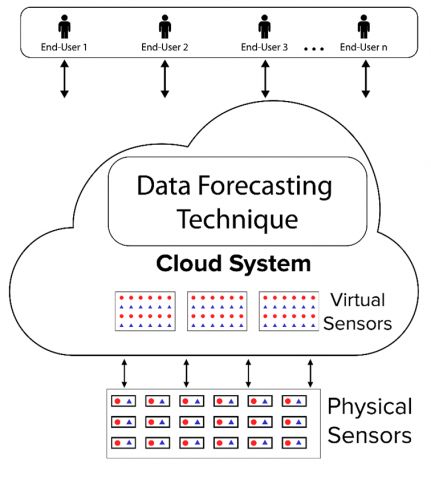
In traditional models, sensor nodes gather data and transmit it to the cloud system so that the users get the information. As the sensor node of the WSN collects data every 10 minutes, and in the traditional approach, the node must send data every 10 minutes to the cloud, which will consume more energy. In our proposed method, the sensor nodes transmit with the cloud every 110 minutes as the prediction technique within the cloud system forecasts ten steps ahead forecasted value. We have used ARIMA, WBF, and ARIMA-WBF as the forecasting techniques. The accuracy of the ARIMA model is better compare to others. Due to less transmission of data from the sensors to the cloud, the proposed method is energy efficient. The proposed model for the energy-efficient sensor cloud using the data prediction approach is shown in Figure 1.
Figure 1. Data prediction-based energy-efficient sensor cloud
2.1 Data and preliminary analysis
2.1.1 Sensor datasets
Nine sensors’ datasets [29] deployed at Library at the Dock and Fitzroy Gardens, Sidney, are used for the simulation. The environmental sensor measuring humidity, light levels, and temperature are analyzed. The data is collected every 10 min from 15/12/2014 to 20/05/2015 for all the nine sensors having three measurements, respectively.
In total twenty-seven environmental sensor datasets are collected for measuring humidity, light levels, and temperature, respectively. Table 1 shows the nine environmental sensor data sets' descriptions for measuring humidity, light levels, and temperature, respectively.
Table 1. Descriptions of sensor data sets of humidity, light, and temperature
|
Sensor |
Data |
No. of Data |
Min Value |
Max Value |
Mean |
1st Quartile |
Median |
3rd Quartile |
|
1 |
Humidity (H1) |
6626 |
7.00 |
74.30 |
46.12 |
38.50 |
48.60 |
56.30 |
|
|
Light (L1) |
6626 |
4.50 |
98.20 |
36.56 |
7.80 |
8.50 |
89.00 |
|
|
Temperature (T1) |
6626 |
4.50 |
42.60 |
16.88 |
13.20 |
16.50 |
19.40 |
|
2 |
Humidity (H2) |
12038 |
19.10 |
69.10 |
48.39 |
42.50 |
49.20 |
54.90 |
|
|
Light (L2) |
12038 |
0.60 |
98.40 |
50.30 |
1.50 |
73.75 |
95.90 |
|
|
Temperature (T2) |
12038 |
4.20 |
45.20 |
18.09 |
13.90 |
17.10 |
21.90 |
|
3 |
Humidity (H3) |
19119 |
1.50 |
68.60 |
53.53 |
46.10 |
56.20 |
63.00 |
|
|
Light (L3) |
19119 |
1.50 |
98.40 |
47.44 |
2.90 |
29.10 |
95.70 |
|
|
Temperature (T3) |
19119 |
5.20 |
41.30 |
18.18 |
14.20 |
17.40 |
21.30 |
|
4 |
Humidity (H4) |
2902 |
1.90 |
102.5 |
44.31 |
35.10 |
47.30 |
60.40 |
|
|
Light (L4) |
2902 |
0.00 |
98.00 |
55.60 |
1.10 |
88.20 |
96.00 |
|
|
Temperature (T4) |
2902 |
8.40 |
37.10 |
19.86 |
16.10 |
19.00 |
23.50 |
|
5 |
Humidity (H5) |
2727 |
7.00 |
67.70 |
42.27 |
33.50 |
43.30 |
50.80 |
|
|
Light (L5) |
2727 |
0.80 |
97.30 |
54.48 |
1.90 |
83.25 |
93.40 |
|
|
Temperature (T5) |
2727 |
9.70 |
34.50 |
19.91 |
16.80 |
19.00 |
22.30 |
|
6 |
Humidity (H6) |
2914 |
11.40 |
76.50 |
50.38 |
42.10 |
51.00 |
59.00 |
|
|
Light (L6) |
2914 |
1.90 |
98.00 |
52.08 |
2.90 |
78.30 |
91.10 |
|
|
Temperature (T6) |
2914 |
11.00 |
35.80 |
20.42 |
17.70 |
20.00 |
22.90 |
|
7 |
Humidity (H7) |
2917 |
10.00 |
76.50 |
47.53 |
37.40 |
48.30 |
57.40 |
|
|
Light (L7) |
2917 |
0.40 |
98.30 |
55.15 |
0.90 |
86.80 |
95.50 |
|
|
Temperature (T7) |
2917 |
9.70 |
34.80 |
19.73 |
16.50 |
19.00 |
22.60 |
|
8 |
Humidity (H8) |
2724 |
10.90 |
74.90 |
48.68 |
39.30 |
49.90 |
57.60 |
|
|
Light (L8) |
2724 |
1.90 |
97.80 |
54.33 |
3.10 |
84.60 |
94.00 |
|
|
Temperature (T8) |
2724 |
8.70 |
36.8 |
19.03 |
16.10 |
18.10 |
21.90 |
|
9 |
Humidity (H9) |
4597 |
9.80 |
74.3 |
48.43 |
41.42 |
50.20 |
56.70 |
|
|
Light (L9) |
4597 |
6.50 |
98.7 |
49.59 |
10.90 |
13.55 |
96.00 |
|
|
Temperature (T9) |
4597 |
5.80 |
43.9 |
19.51 |
16.10 |
18.70 |
21.90 |
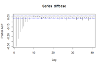
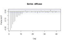
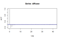
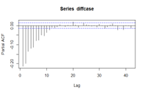
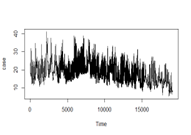
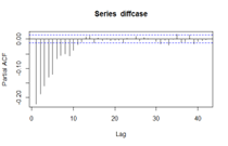
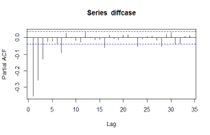
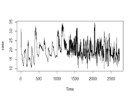
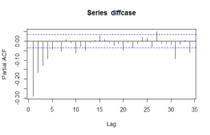
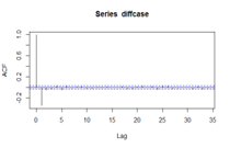
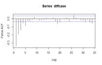
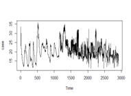
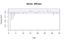
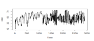
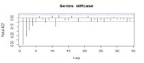
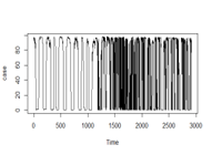
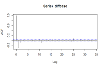
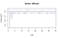
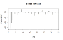
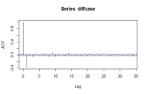
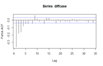
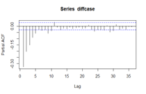
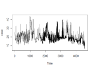
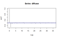
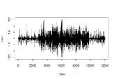
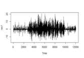
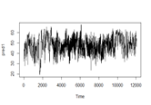
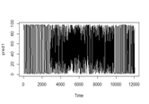
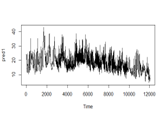
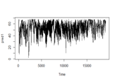
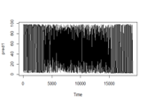
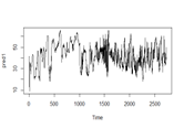
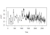
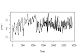
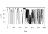
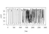
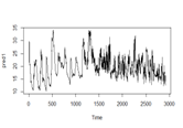
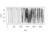
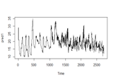
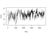
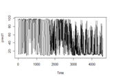
Table 2. Training sensor data sets of humidity, light, and temperature and the ACF, PACF graphs for twenty-seven univariate time-series data
|
Data |
Training Data |
ACF Graph |
PACF Graph |
|
H1 |
|||
|
L1 |
|||
|
T1 |
|||
|
H2 |
|||
|
L2 |
|||
|
T2 |
|||
|
H3 |
|||
|
L3 |
|||
|
T3 |
|||
|
H4 |
|||
|
L4 |
|||
|
T4 |
|||
|
H5 |
|||
|
L5 |
|||
|
T5 |
|||
|
H6 |
|||
|
L6 |
|||
|
T6 |
|||
|
H7 |
|||
|
L7 |
|||
|
T7 |
|||
|
H8 |
|||
|
L8 |
|||
|
T8 |
|||
|
H9 |
|||
|
L9 |
|||
|
T9 |
2.1.2 Basic data analysis
A summary of the environmental sensor data sets for measuring humidity, light levels, and temperature are shown in Table 1.
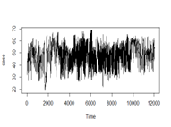
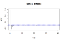
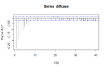
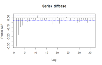
Table 2 shows these twenty-seven sensor datasets for measuring humidity, light levels, and the temperature started with different 10 min, and these environmental curves not showing non-linear nature. We bound our attention to trend and linear models. To fit the individual conventional ARIMA model and ARIMA-WBF model, the parameters, namely $p$ and $q$, are specified by plotting PACF and ACF plots (see Table 2).
2.1.3 Performance evaluation metrics
The mean absolute error (MAE) and root mean square error (RMSE) are used to evaluate [30] the performance of different forecasting models for the sensor data sets. The mathematical expressions are explained as follows:
$R M S E=\sqrt{\frac{1}{n} \sum_{i=1}^n\left(y_i-\hat{y}_i\right)^2}$ (2)
$M A E=\frac{1}{n} \sum_{i=1}^n\left|y_i-\hat{y}_i\right|$ (3)
where, $\hat{y}_i$ is the predicted output and $y_i$ is the actual output.
2.2 Methodology
We have used ARIMA, WBF, and ARIMA-WBF as the forecasting techniques. We have used the combination of ARIMA and WBF methods to forecast the environmental sensor for measuring humidity, light levels, and temperature.
2.2.1 ARIMA model
The ARIMA model [31] is a linear regression model. The ARIMA (p, d, q), where the model structure is decided by p, d, and q integer parameter values. The ARIMA model [32] is mathematically expressed as follows:
$\begin{gathered}y_t=\theta_0+\varphi_1 y_{t-1}+\varphi_2 y_{t-2}+\cdots+\varphi_p y_{t-p}+\varepsilon_t- \theta_1 \varepsilon_{t-1}+\theta_2 \varepsilon_{t-2}+\cdots+\theta_q \varepsilon_{t-q}\end{gathered}$ (4)
where, the random error at time t is $\varepsilon_t$, the actual value is $y_t, \varphi_i$ and $\theta_j$ are the model's coefficients. It is assumed that $\varepsilon_{t-1}\left(\varepsilon_{t-1}=y_{t-1}-\hat{y}_{t-1}\right)$ has constant variance and zero mean. The methods consist of the following three iterative steps: (1) The model Identification, (2) estimation of the parameters, (3) using the residual analysis for checking the model to get the best fitted. In the first step differencing is applied to make the data stationary. Once the data is stationary, the partial autocorrelation function (PACF) and the autocorrelation function (ACF) graph are analyzed to select the MA and AR model types. The Akaike Information Criterion (AIC) is used for the estimation of parameters. At last, residual analysis is carried out to check the model to get the best-fitted model. ARIMA model generally does not perform well in non-linear data sets, so in the next session, we have discussed the WBF model.
2.2.2 WBF model
Generally, the wavelet models are used in nonstationary datasets, unlike ARIMA [33]. Most climatic and epidemic time-series analysis of datasets are nonstationary; thus, the wavelet model [34, 35] is mostly used to forecast. The selection of the optimal number of decomposition level in the WBF model is as follows:
$W_L=\operatorname{int}[\log (m)]$ (5)
where, m is the time-series length. The working principle of a wavelet-based forecasting model is explained by Messina et al. [34]. Daubechies wavelets can generate events in so many fashions across the observed time series that most other time series forecasting models cannot recognize [36].
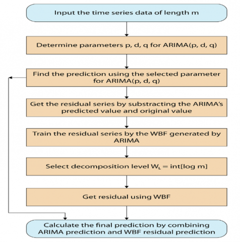
2.2.3 ARIMA-WBF model
Figure 2. Flow chart for the hybrid ARIMA-WBF model
For the environmental sensor datasets, a combination of the stationary ARIMA and WBF model, which is nonstationary in nature, reduces the component models' individual biases. The present sensor datasets for twenty-seven univariate time series are linear. If it is non-linear, then the ARIMA model fails to produce random errors. The current sensor datasets are linear. We have used a hybrid model for proving this practically, which is a combination of WBF and ARIMA. The wavelet function is chosen to model the residual series generated from the ARIMA model. Several hybrids [37, 38] models using ARIMA and neural networks. The algorithm of the hybrid ARIMA-WBF model is described in Figure 2.
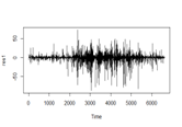
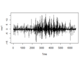
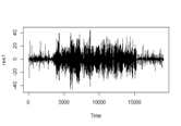
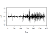
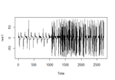
It is challenging to study the limited environmental sensor nine datasets' characteristics and nature of measuring humidity, light, and temperature. So, we consider one significant problem relevant to the environmental sensor datasets for a total of twenty-seven sensor datasets. This paper deals with the data-driven forecasts of the ten-minute sensor datasets of measuring humidity, light, and temperature. We have used a novel parsimonious ARIMA model of the twenty-seven sensor datasets. Hundred minutes ahead (short-term) out of sample forecasts is predicted for these twenty-seven datasets. Twenty-seven univariate time series sensor datasets of humidity, light, and temperature are used to train the hybrid model and the traditional constituent models. The datasets are linear, nonstationary, and statistical tests confirmed this. We experimentally evaluate ARIMA, WBF, and hybrid ARIMA-WBF models for all these twenty-seven sensor datasets. We have used MAE and RMSE for the evaluation of the predictive performance [39] of the models.We start evaluating our experiment for the twenty-seven univariate ten min time series datasets with the ARIMA model using the 'forecast’ [40] package in R. We fit the wavelet model using the ARIMA function. Once the ARIMA is fitted, predictions are generated ten steps ahead for short-term forecasts for all the twenty-seven sensor datasets measuring humidity, light, and temperature. We compute the predicted values of training data and analyze the residual errors using traditional and advanced individual models, namely ARIMA and the hybrid ARIMA-WBF model. Plots of the residual series are given in Table 3.
Table 3. Plots of residuals and predicted values of sensor data sets for ARIMA model for humidity, light, and temperature
|
Value |
Sensor Data |
Humidity (H) |
Light (L) |
Temperature (T) |
|
Residual |
1 |
|||
|
Predicted |
1 |
|||
|
Residual |
2 |
|||
|
Predicted |
2 |
|||
|
Residual |
3 |
|||
|
Predicted |
3 |
|||
|
Residual |
4 |
|||
|
Predicted |
4 |
|||
|
Residual |
5 |
|||
|
Predicted |
5 |
|||
|
Residual |
6 |
|||
|
Predicted |
6 |
|||
|
Residual |
7 |
|||
|
Predicted |
7 |
|||
|
Residual |
8 |
|||
|
Predicted |
8 |
|||
|
Residual |
9 |
|||
|
Predicted |
9 |
Table 4. ARIMA models of sensor data sets of humidity, light and temperature
|
Sensor Data |
ARIMA (p,d,q) |
ARIMA Model |
|
H1 |
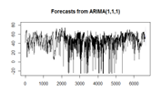
(1,1,1) |
$\widehat{\Delta y}_t=0.2295 \widehat{\Delta y}_{t-1}-0.7168 \hat{\varepsilon}_{t-1}$ |
|
L1 |
(2,1,1) |
$\widehat{\Delta y}_t=0.3037 \widehat{\Delta y}_{t-1}+0.0615 \widehat{\Delta y}_{t-2}-0.7158 \hat{\varepsilon}_{t-1}$ |
|
T1 |
(0,1,2) |
$\widehat{\Delta y}_t=-0.4163 \hat{\varepsilon}_{t-1}-0.0897 \hat{\varepsilon}_{t-2}$ |
|
H2 |
(3,1,1) |
$\widehat{\Delta y}_t=0.3232 \widehat{\Delta y}_{t-1}-0.0026 \widehat{\Delta y}_{t-2}+0.0195 \widehat{\Delta y}_{t-3}-0.7486 \hat{\varepsilon}_{t-1}$ |
|
L2 |
(1,1,2) |
$\widehat{\Delta y}_t=0.3036 \widehat{\Delta y}_{t-1}-0.6928 \hat{\varepsilon}_{t-1}-0.0423 \hat{\varepsilon}_{t-2}$ |
|
T2 |
(0,1,3) |
$\widehat{\Delta y}_t=-0.4364 \hat{\varepsilon}_{t-1}-0.1527 \hat{\varepsilon}_{t-2}-0.0329 \hat{\varepsilon}_{t-3}$ |
|
H3 |
(2,1,2) |
$\widehat{\Delta y}_t=0.0009+0.9188 \widehat{\Delta y}_{t-1}-0.2583 \widehat{\Delta y}_{t-2}-1.2571 \hat{\varepsilon}_{t-1}+0.3738 \hat{\varepsilon}_{t-2}$ |
|
L3 |
(1,1,2) |
$\widehat{\Delta y}_t=0.3940 \widehat{\Delta y}_{t-1}-0.7289 \hat{\varepsilon}_{t-1}-0.0727 \hat{\varepsilon}_{t-2}$ |
|
T3 |
(2,1,2) |
$\widehat{\Delta y}_t=1.1458 \widehat{\Delta y}_{t-1}-0.3685 \widehat{\Delta y}_{t-2}-1.4940 \hat{\varepsilon}_{t-1}+0.5721 \hat{\varepsilon}_{t-2}$ |
|
H4 |
(1,1,2) |
$\widehat{\Delta y}_t=0.9150 \widehat{\Delta y}_{t-1}-1.3709 \hat{\varepsilon}_{t-1}+0.3877 \hat{\varepsilon}_{t-2}$ |
|
L4 |
(1,0,2) |
$\widehat{\Delta y}_t=55.5964+0.9448 \widehat{\Delta y}_{t-1}-0.3933 \hat{\varepsilon}_{t-1}-0.0683 \hat{\varepsilon}_{t-2}$ |
|
T4 |
(2,1,1) |
$\widehat{\Delta y}_t=0.0040 \widehat{\Delta y}_{t-1}-0.0987 \widehat{\Delta y}_{t-2}-0.4868 \hat{\varepsilon}_{t-1}$ |
|
H5 |
(1,1,2) |
$\widehat{\Delta y}_t=0.5239 \widehat{\Delta y}_{t-1}-0.8898 \hat{\varepsilon}_{t-1}+0.0981 \hat{\varepsilon}_{t-2}$ |
|
L5 |
(1,0,2) |
$\widehat{\Delta y}_t=54.4748+0.9494 \widehat{\Delta y}_{t-1}-0.4222 \hat{\varepsilon}_{t-1}-0.0952 \hat{\varepsilon}_{t-2}$ |
|
T5 |
(1,1,1) |
$\widehat{\Delta y}_t=0.2480 \widehat{\Delta y}_{t-1}-0.6649 \hat{\varepsilon}_{t-1}$ |
|
H6 |
(2,1,2) |
$\widehat{\Delta y}_t=-0.0075 \widehat{\Delta y}_{t-1}+0.1346 \widehat{\Delta y}_{t-2}-0.3735 \hat{\varepsilon}_{t-1}-0.2404 \hat{\varepsilon}_{t-2}$ |
|
L6 |
(1,0,2) |
$\widehat{\Delta y}_t=52.0821+0.9490 \widehat{\Delta y}_{t-1}-0.4210 \hat{\varepsilon}_{t-1}-0.0643 \hat{\varepsilon}_{t-2}$ |
|
T6 |
(3,1,1) |
$\widehat{\Delta y}_t=0.0593 \widehat{\Delta y}_{t-1}-0.0173 \widehat{\Delta y}_{t-2}-0.0561 \widehat{\Delta y}_{t-3}-0.5477 \hat{\varepsilon}_{t-1}$ |
|
H7 |
(2,1,1) |
$\widehat{\Delta y}_t=0.2243 \widehat{\Delta y}_{t-1}-0.0337 \widehat{\Delta y}_{t-2}-0.6424 \hat{\varepsilon}_{t-1}$ |
|
L7 |
(2,0,4) |
$\widehat{\Delta y}_t=55.1164+1.9534 \widehat{\Delta y}_{t-1}-0.9565 \widehat{\Delta y}_{t-2}-1.4398 \hat{\varepsilon}_{t-1}+0.4138 \hat{\varepsilon}_{t-2}-0.0 .0419 \hat{\varepsilon}_{t-3}+0.0822 \hat{\varepsilon}_{t-4}$ |
|
T7 |
(2,1,2) |
$\widehat{\Delta y}_t=-0.0042 \widehat{\Delta y}_{t-1}+0.0324 \widehat{\Delta y}_{t-2}-0.4084 \hat{\varepsilon}_{t-1}-0.1645 \hat{\varepsilon}_{t-2}$ |
|
H8 |
(3,1,2) |
$\widehat{\Delta y}_t=-0.5797 \widehat{\Delta y}_{t-1}+0.0948 \widehat{\Delta y}_{t-2}-0.0442 \widehat{\Delta y}_{t-3}+0.1462 \hat{\varepsilon}_{t-1}-0.4148 \hat{\varepsilon}_{t-2}$ |
|
L8 |
(1,0,2) |
$\widehat{\Delta y}_t=54.3273+0.9464 \widehat{\Delta y}_{t-1}-0.4072 \hat{\varepsilon}_{t-1}-0.0815 \hat{\varepsilon}_{t-2}$ |
|
T8 |
(3,1,1) |
$\widehat{\Delta y}_t=0.0714 \widehat{\Delta y}_{t-1}-0.0261 \widehat{\Delta y}_{t-2}-0.0679 \widehat{\Delta y}_{t-3}-0.5506 \hat{\varepsilon}_{t-1}$ |
|
H9 |
(1,1,1) |
$\widehat{\Delta y}_t=0.2360 \widehat{\Delta y}_{t-1}-0.6570 \hat{\varepsilon}_{t-1}$ |
|
L9 |
(1,1,1) |
$\widehat{\Delta y}_t=0.2705 \widehat{\Delta y}_{t-1}-0.7163 \hat{\varepsilon}_{t-1}$ |
|
T9 |
(1,1,1) |
$\widehat{\Delta y}_t=0.2326 \widehat{\Delta y}_{t-1}-0.6177 \hat{\varepsilon}_{t-1}$ |
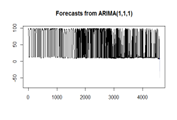
The ARIMA residual forecasts and WBF forecasts are added to find the out-of-sample forecasts using the hybrid ARIMA-WBF model for the next ten steps ahead. The best fitted parsimonious ARIMA models of twenty-seven environmental sensor datasets measuring humidity, light, and temperature are presented in Table 4.
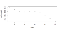
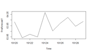
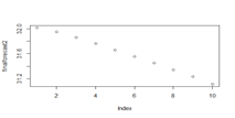
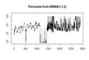
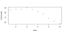
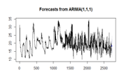
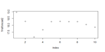
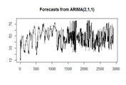
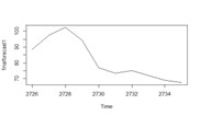
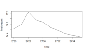
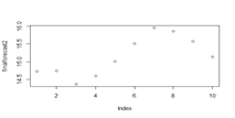
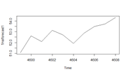
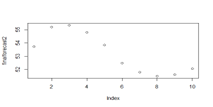
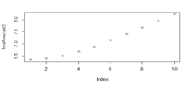
The real-time forecasted values of sensor data sets for the ARIMA model, out of sample Real-time (short-term) forecasts (hundred ten minutes ahead) of sensor data sets for both ARIMA and hybrid ARIMA-WBF models are displayed in Table 5.
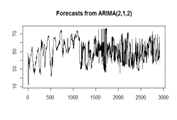
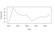
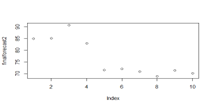
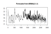
Table 5. Forecasted values of sensor data sets for the ARIMA model, out of real-time sample forecasts (10 ten steps ahead) of sensor data sets for both ARIMA and hybrid ARIMA-WBF models
|
Sensor Data |
Forecasted Value by ARIMA |
ARIMA 10 Step ahead |
Hybrid ARIMA-WBF 10 Step ahead |
|
H1 |
|||
|
L1 |
|||
|
T1 |
|||
|
H2 |
|||
|
L2 |
|||
|
T2 |
|||
|
H3 |
|||
|
L3 |
|||
|
T3 |
|||
|
H4 |
|||
|
L4 |
|||
|
T4 |
|||
|
H5 |
|||
|
L5 |
|||
|
T5 |
|||
|
H6 |
|||
|
L6 |
|||
|
T6 |
|||
|
H7 |
|||
|
L7 |
|||
|
T7 |
|||
|
H8 |
|||
|
L8 |
|||
|
T8 |
|||
|
H9 |
|||
|
L9 |
|||
|
T9 |
We applied an advanced hybrid ARIMA-WBF model for the nonlinearity, nonstationarity, and non-Gaussian environmental sensor datasets of measuring humidity, light, and temperature for comparison purposes. The results of the simulations are displayed in Table 6. Our proposed individual ARIMA model performance is better than the hybrid model in twenty-one out of twenty-seven datasets of sensor datasets. The RMSE and MAE values are lower in ARIMA compared to the other two models in 78 percent of datasets which signifies the forecasting accuracy of ARIMA is better in most of the cases.
In the simulation, 100 nodes are distributed uniformly in a square of side 100 meters. The rate of the data flow of all the nodes is 40Kbps. And the sink is at the left corner of the square. We have calculated the energy consumption by forwarding the network traffic using the shortest path algorithm to reach the sink. list of parameters used in the simulation is explained in Table 7.
Table 6. The performance in terms of quantitative measures for various prediction models on twenty-seven sensor datasets for humidity, light, and temperature
|
|
Performance |
|||||||||
|
Model |
|
H1 |
L1 |
T1 |
H2 |
L2 |
T2 |
H3 |
L3 |
T3 |
|
RMSE |
|
|
|
|
|
|
|
|
|
|
|
ARIMA |
|
8.8 |
23.7 |
2.1 |
4.63 |
28.39 |
2.93 |
5.9 |
27.04 |
2.33 |
|
WBF |
|
9.4 |
24.6 |
2.2 |
4.72 |
33.94 |
3.19 |
7.2 |
37.59 |
3.29 |
|
ARIMA-WBF |
|
9.5 |
25.7 |
2.8 |
5.01 |
30.72 |
3.16 |
6.4 |
29.17 |
2.52 |
|
|
|
H1 |
L1 |
T1 |
H2 |
L2 |
T2 |
H3 |
L3 |
T3 |
|
Model |
MAE |
|
|
|
|
|
|
|
|
|
|
ARIMA |
|
4.77 |
12.25 |
1.16 |
2.84 |
15.1 |
1.74 |
3.54 |
15.04 |
1.35 |
|
WBF |
|
5.32 |
13.39 |
1.24 |
3.01 |
26.7 |
1.96 |
5.10 |
31.15 |
2.42 |
|
ARIMA-WBF |
|
5.18 |
14.13 |
1.27 |
3.04 |
17.9 |
1.85 |
3.78 |
16.26 |
1.43 |
|
|
Performance |
|||||||||
|
Model |
|
H4 |
L4 |
T4 |
H5 |
L5 |
T5 |
H6 |
L6 |
T6 |
|
RMSE |
|
|
|
|
|
|
|
|
|
|
|
ARIMA |
|
10.65 |
25.01 |
2.58 |
5.52 |
25.04 |
2.1 |
5.65 |
23.32 |
1.94 |
|
WBF |
|
10.83 |
27.07 |
3.30 |
5.64 |
27.28 |
2.2 |
5.80 |
24.58 |
2.58 |
|
ARIMA-WBF |
|
11.43 |
26.96 |
2.87 |
6.23 |
27.11 |
2.4 |
6.30 |
25.63 |
2.19 |
|
Model |
|
H4 |
L4 |
T4 |
H5 |
L5 |
T5 |
H6 |
L6 |
T6 |
|
MAE |
|
|
|
|
|
|
|
|
|
|
|
ARIMA |
|
5.77 |
14.53 |
1.53 |
3.24 |
15.0 |
1.2 |
3.20 |
13.54 |
1.12 |
|
WBF |
|
5.89 |
14.10 |
2.45 |
3.44 |
14.6 |
1.3 |
3.43 |
13.36 |
1.91 |
|
ARIMA-WBF |
|
5.74 |
13.93 |
1.64 |
3.58 |
14.9 |
1.4 |
3.55 |
13.59 |
1.12 |
|
|
Performance |
|||||||||
|
Model |
|
H7 |
L7 |
T7 |
H8 |
L8 |
T8 |
H9 |
L9 |
T9 |
|
|
RMSE |
|
|
|
|
|
|
|
|
|
|
ARIMA |
|
6.67 |
24.61 |
2.29 |
5.94 |
24.8 |
2.2 |
6.08 |
25.13 |
2.55 |
|
WBF |
|
7.25 |
25.39 |
3.01 |
6.11 |
25.6 |
2.7 |
6.21 |
27.09 |
2.61 |
|
ARIMA-WBF |
|
7.34 |
26.89 |
2.51 |
6.58 |
27.0 |
2.5 |
6.61 |
27.21 |
2.76 |
|
Model |
|
H7 |
L7 |
T7 |
H8 |
L8 |
T8 |
H9 |
L9 |
T9 |
|
MAE |
|
|
|
|
|
|
|
|
|
|
|
ARIMA |
|
3.83 |
14.16 |
1.36 |
3.54 |
14.7 |
1.35 |
3.63 |
13.77 |
1.43 |
|
WBF |
|
4.35 |
13.41 |
2.23 |
3.80 |
13.7 |
2.02 |
3.87 |
15.29 |
1.54 |
|
ARIMA-WBF |
|
4.36 |
14.72 |
1.51 |
4.01 |
13.7 |
1.48 |
4.00 |
15.62 |
1.59 |
Table 7. List of parameters
|
Parameters |
Values/Unit |
|
No of Sensor Nodes |
100 |
|
Area of Simulation |
100 * 100 square meter |
|
Types of Communication |
Multi-hop |
|
Nodes Distribution |
Uniform |
|
Simulation Time |
100 Hours |
|
Data Rate |
40Kbps |
|
Transmission Range |
20 Meter |
|
σ |
4 |
|
Gateway Position |
Corner of the square |
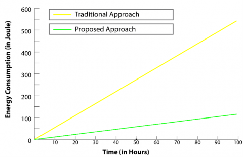
Figure 3. The energy consumption in the proposed and traditional method
In the conventional approach, sensor nodes send data every 10 minutes to cloud systems as data is collected every 10 minutes. In the proposed approach, ten steps ahead forecasting is used in the cloud system, so sensors send data every 110 minutes to the cloud. The power consumption in the proposed and traditional approach is explained in Figure 3. In the traditional method, sensor nodes send data every 10 minutes to cloud systems as data is collected every 10 minutes. In the proposed approach, ten steps ahead forecasting is used in the cloud system, so sensors send data every 110 minutes to the cloud.
It is observed that the proposed methods consume less energy as compared to the traditional method for the sensor cloud system.
This paper used the ARIMA-WBF model using residual modelling for humidity, light, and temperature forecasting for the sensor data 1 to 9. The ARIMA-WBF model explains the non-linear, linear, and nonstationary tendencies present in the humidity, light, and temperature data sets of nine different sensors. Since all the data sets are linearity and nonstationarity, the proposed ARIMA model can perform better than the other two models. It also provides better accuracy in forecasting than other advanced models like WBF and ARIMA-WBF for twenty-seven out of twenty-seven data sets under RMSE and twenty-one out of twenty-seven data sets under MAE of humidity, light, and temperature, respectively considered in this study. The present model can forecast with better accuracy if the linearity of the ARIMA model is satisfied. Ten minutes for ten steps ahead of sample forecasts are provided separately for twenty-seven environmental sensor datasets measuring humidity, light, and temperature. As the sensor node of the WSN collects data every 10 minutes, and in the traditional approach node and sends data every 10 minutes to the cloud, which will consume more energy. In our proposed approach, the sensor nodes communicate with the cloud every 110 minutes as the forecasting technique within the cloud system forecasts the ten steps ahead forecasted value. We have used ARIMA, WBF, and ARIMA-WBF as the forecasting techniques. Our results show the accuracy of the ARIMA model is better compare to others.
A Sensor-Cloud using the data forecasting technique is proposed, which is energy efficient. We have used ARIMA, WBF, and ARIMA-WBF as the forecasting techniques. Our results show the accuracy of the ARIMA model is better compare to others. The sensor nodes gather data and send it to the cloud system. The end users get the sensor information from the cloud. As the sensor node of the WSN collects data every 10 minutes, and in the traditional approach, the node must send data every 10 minutes to the cloud, which will consume more energy. In our proposed approach, the sensor nodes transmit data to the cloud every 110 minutes as the forecasting technique within the cloud system forecasts the ten steps ahead forecasted value. Due to less transmission of data to the cloud from the sensors, the proposed approach is energy efficient. Our proposed method consumes 0.090909 times lower power as compared to existing methods in the sensor cloud due to less data transmission, and the RMSE and MAE in the prediction are also significantly less.
[1] Misra, S., Chatterjee, S., Obaidat, M.S. (2014). On theoretical modeling of sensor cloud: A paradigm shift from wireless sensor network. IEEE Systems Journal, 11(2): 1084-1093. https://doi.org/10.1109/JSYST.2014.2362617
[2] Yuriyama, M., Kushida, T. (2010). Sensor-cloud infrastructure-physical sensor management with virtualized sensors on cloud computing. International Conference on Network-Based Information Systems, Takayama, Japan, pp. 1-8. https://doi.org/10.1109/NBiS.2010.32
[3] Alamri, A., Ansari, W.S., Hassan, M.M., Hossain, M.S., Alelaiwi, A., Hossain, M.A. (2013). A survey on sensor-cloud: architecture, applications, and approaches. International Journal of Distributed Sensor Networks, 9(2): 1-18. https://doi.org/10.1155/2013/917923
[4] You, P., Li, H., Peng, Y., Li, Z. (2013). An integration framework of cloud computing with wireless sensor networks. Ubiquitous Information Technologies and Applications, Xi'an, China, pp. 381-387. https://doi.org/10.1007/978-94-007-5857-5_41
[5] Dinh, T., Kim, Y. (2016). An efficient interactive model for on-demand sensing-as-a-services of sensor-cloud. Sensors, 16(7): 49-59. https://doi.org/10.1016/j.engappai.2017.07.007
[6] Lemos, M., Rabelo, R., Mendes, D., Carvalho, C., Holanda, R. (2019). An approach for provisioning virtual sensors in sensor clouds. International Journal of Network Management, 29(2): 1-21. https://doi.org/10.1002/nem.2062
[7] Das, K., Das, S., Darji, R.K., Mishra, A. (2018). Survey of energy-efficient techniques for the cloud-integrated sensor network. Journal of Sensors, 2018: 1-17. https://doi.org/10.1155/2018/1597089
[8] Guha, R.K., Gunter, C.A., Sarkar, S. (2006). Fair coalitions for power-aware routing in wireless networks. IEEE Transactions on Mobile Computing, 6(2): 206-220. https://doi.org/10.1109/TMC.2007.27
[9] Anjali, T., Chandini, K., Anoop, K., Lajish, V.L. (2019). Temperature prediction using machine learning approaches, International Conference on Intelligent Computing, Instrumentation and Control Technologies, Kannur, India, pp. 1264-1268. https://doi.org/10.1109/ICICICT46008.2019.8993316
[10] Chu, W.T., Ho, K.C., Borji, A. (2018). Visual weather temperature prediction. In Winter Conference on Applications of Computer Vision, Lake Tahoe, NV, USA, pp. 234-241. https://doi.org/10.1109/WACV.2018.00032
[11] Kisi, O., Shiri, J. (2014). Prediction of long‐term monthly air temperature using geographical inputs. International Journal of Climatology, 34(1): 179-186. https://doi.org/10.1002/joc.3676
[12] Afroz, Z., Shafiullah, G.M., Urmee, T., Higgins, G. (2017). Prediction of indoor temperature in an institutional building. Energy Procedia, 142: 1860-1866. https://doi.org/10.1016/j.egypro.2017.12.576
[13] Park, I., Kim, H.S., Lee, J., Kim, J.H., Song, C.H., Kim, H.K. (2019). Temperature prediction using the missing data refinement model based on a long short-term memory neural network. Atmosphere, 10(11): 1-16. https://doi.org/10.3390/atmos10110718
[14] Krishnaveni, N., Padma, A. (2021). Weather forecast prediction and analysis using sprint algorithm. Journal of Ambient Intelligence and Humanized Computing, 12: 4901-4909. https://doi.org/10.1007/s12652-020-01928-w
[15] Yang, L., Shang, L., Yang, L. (2016). Improved prediction of Markov chain algorithm for indoor temperature. In International Symposium on Computer, Consumer and Control, Xi'an, China, pp. 809-812. https://doi.org/10.1109/IS3C.2016.206
[16] Panigrahi, S., Behera, H.S. (2017). A hybrid ETS–ANN model for time series forecasting. Engineering Applications of Artificial Intelligence, 66: 49-59. https://doi.org/10.1016/j.engappai.2017.07.007
[17] Panigrahi, S., Behera, H.S. (2019). Nonlinear time series forecasting using a novel self-adaptive TLBO-MFLANN model. International Journal of Computational Intelligence Studies, 8(1-2): 4-26. https://doi.org/10.1504/IJCISTUDIES.2019.098013
[18] Pattanayak, R.M., Panigrahi, S., Behera, H.S. (2020). High-order fuzzy time series forecasting by using membership values along with data and support vector machine. Arabian Journal for Science and Engineering, 45(12): 10311-10325. https://doi.org/10.1007/s13369-020-04721-1
[19] Panigrahi, S., Behera, H.S. (2020). Time series forecasting using differential evolution-based ANN modelling scheme. Arabian Journal for Science and Engineering, 45(12): 11129-11146. https://doi.org/10.1007/s13369-020-05004-5
[20] Izonin, I., Tkachenko, R., Verhun, V., Zub, K. (2021). An approach towards missing data management using improved GRNN-SGTM ensemble method. Engineering Science and Technology, an International Journal, 24(3): 749-759. https://doi.org/10.1016/j.jestch.2020.10.005
[21] Valente, J.M., Maldonado, S. (2020). SVR-FFS: A novel forward feature selection approach for high-frequency time series forecasting using support vector regression. Expert Systems with Applications, 160: 1-13. https://doi.org/10.1016/j.eswa.2020.113729
[22] Dantas, T.M., Oliveira, F.L.C. (2018). Improving time series forecasting: An approach combining bootstrap aggregation, clusters and exponential smoothing. International Journal of Forecasting, 34(4): 748-761. https://doi.org/10.1016/j.ijforecast.2018.05.006
[23] Deng, Y.F., Jin, X., Zhong, Y.X. (2005). Ensemble SVR for prediction of time series. In International Conference on Machine Learning and Cybernetics, Guangzhou, China, pp. 3528-3534. https://doi.org/10.1109/ICMLC.2005.1527553
[24] Jaseena, K.U., Kovoor, B.C. (2022). Deterministic weather forecasting models based on intelligent predictors: A survey. Journal of King Saud University-Computer and Information Sciences, 34(6): 3393-3412. https://doi.org/10.1016/j.jksuci.2020.09.009
[25] Baydilli, Y., Atila, U. (2018). Understanding effects of hyper-parameters on learning: A comparative analysis. International Conference on Advanced Technologies, Computer Engineering and Science, Safranbolu, Turkey, pp. 11-13.
[26] Fay, D., Ringwood, J. (2007). A wavelet transfer model for time series forecasting. International Journal of Bifurcation and Chaos, 17(10): 3691-3696. https://doi.org/10.1142/S0218127407019585
[27] Aminghafari, M., Poggi, J.M. (2007). Forecasting time series using wavelets. International Journal of Wavelets, Multiresolution and Information Processing, 5(5): 709-724. https://doi.org/10.1142/S0219691307002002
[28] Nury, A.H., Hasan, K., Alam, M.J.B. (2017). Comparative study of wavelet-ARIMA and wavelet-ANN models for temperature time series data in northeastern Bangladesh. Journal of King Saud University-Science, 29(1): 47-61. https://doi.org/10.1016/j.jksus.2015.12.002
[29] City of Melbourne Open Data Team, https://data.melbourne.vic.gov.au/ Environment/Sensor-readings-with-temperature-light-humidity-ev/ez6b-syvw, accessed on Feb. 25, 2020.
[30] Ahmed, N.K., Atiya, A.F., Gayar, N.E., El-Shishiny, H. (2010). An empirical comparison of machine learning models for time series forecasting. Econometric Reviews, 29(5-6): 594-621. https://doi.org/10.1080/07474938.2010.481556.
[31] Box, G.E., Jenkins, G.M., Reinsel, G.C., Ljung, G.M. (2015). Time Series Analysis: Forecasting and Control. John Wiley & Sons.
[32] Chakraborty, T., Chattopadhyay, S., Ghosh, I. (2019). Forecasting dengue epidemics using a hybrid methodology. Physica A: Statistical Mechanics and its Applications, 527: 1-8. https://doi.org/10.1016/j.physa.2019.121266
[33] Zhang, G.P. (2003). Time series forecasting using a hybrid ARIMA and neural network model. Neurocomputing, 50: 159-175. https://doi.org/10.1016/S0925-2312(01)00702-0
[34] Messina, J.P., Brady, O.J., Scott, T.W., Zou, C., Pigott, D.M., Duda, K.A., Bhatt, S., Katzelnick, L., Howes, R.E., Battle, K.E., Simmons, C.P., Hay, S.I. (2014). Global spread of dengue virus types: Mapping the 70 year history. Trends in Microbiology, 22(3): 138-146. https://doi.org/10.1016/j.tim.2013.12.011
[35] Buczak, A.L., Baugher, B., Moniz, L.J., Bagley, T., Babin, S.M., Guven, E. (2018). Ensemble method for dengue prediction. PloS One, 13(1): 1-23. https://doi.org/10.1371/journal.pone.0189988
[36] Bhatt, S., Gething, P.W., Brady, O.J., et al. (2013). The global distribution and burden of dengue. Nature, 496(7446): 504-507. https://doi.org/10.1038/nature12060
[37] Chakraborty, T., Ghosh, I. (2020). Real-time forecasts and risk assessment of novel coronavirus (COVID-19) cases: A data-driven analysis. Chaos, Solitons & Fractals, 135: 1-10. https://doi.org/10.1016/j.chaos.2020.109850
[38] Fraiha Lopes, R.L., Fraiha, S.G., Gomes, H.S., Lima, V.D., Cavalcante, G.P. (2020). Application of hybrid ARIMA and artificial neural network modelling for electromagnetic propagation: An alternative to the least squares method and ITU recommendation P. 1546-5 for Amazon urbanized cities. International Journal of Antennas and Propagation, 2020: 1-12. https://doi.org/10.1155/2020/8494185
[39] James, G., Witten, D., Hastie, T., Tibshirani, R. (2013). An Introduction to Statistical Learning. New York: Springer. https://doi.org/10.1007/978-1-0716-1418-1
[40] Hyndman, R.J., Athanasopoulos, G., Bergmeir, C., et al. (2020). Package ‘forecast’. https://cran.r-project.org/web/packages/forecast/forecast.pdf.