Ligang Zhang![]() | Bo Wang*
| Bo Wang*![]() | Li Zhu
| Li Zhu![]() | Qiwei Zhu
| Qiwei Zhu![]()
© 2023 IIETA. This article is published by IIETA and is licensed under the CC BY 4.0 license (http://creativecommons.org/licenses/by/4.0/).
OPEN ACCESS
In the fermentation process of Pichia pastoris, inherent non-linearity and significant time-variance characteristics are observed, making pivotal state variables challenging to measure online. In this study, a novel online soft sensor modelling approach for the Pichia pastoris fermentation process is introduced. A just-in-time learning (JITL) technique, driven by a multi-similarity measurement coupled with a moving window (MW) strategy, was employed. Historical data were partitioned into real-time multiple samples via the MW technique. Subsequent sub-windows were then filtered, adopting a cumulative similarity strategy. The k-MI algorithm was utilised for the selection of local auxiliary variables within the MW, leading to the construction of the local weighted partial least squares model (LWPLS) via a multi-similarity metric-driven JITL. The fusion of sub-models was accomplished through double weighted ensemble learning. Predictive outcomes indicated superior performance of the proposed soft sensor model in estimating the cell and product concentration of Pichia pastoris in comparison to alternative models.
Pichia pastoris, soft sensor, ensemble learning, moving window, multi-similarity measurement
Pichia pastoris is a significant research target in the field of pharmaceutical proteins. Compared with other existing expression systems, Pichia pastoris has obvious advantages in the processing of expression products, external secretion, post-translational modification, and glycosylation modification, and has been widely used in the expression of exogenous proteins [1-4]. In order to give full play to Pichia pastoris expression system as an excellent protein expression system, maximize the production efficiency and product quality of Pichia pastoris fermentation to express exogenous proteins, and reduce the production cost [5, 6], it is necessary to conduct dynamic regulation and real-time optimization of the fermentation process of Pichia pastoris, so as to accurately control the production under the optimal technological conditions. However, the fermentation process of Pichia pastoris has the characteristics of multi-variable, strong coupling and nonlinear [4]. Due to the actual technology and cost, the key parameters that can directly reflect the quality of Pichia pastoris, such as cell concentration, substrate concentration and product concentration, are difficult to be directly measured online. In the absence of cost-effective online detection methods, most use off-line sampling and analysis methods, which makes Pichia pastoris extremely vulnerable to contamination and causes the entire fermentation process to fail. In addition, the off-line laboratory analysis steps are tedious, the data collection interval is long, the lag is large, the real-time performance is poor, these problems become the technical bottleneck of optimization control for the fermentation process of Pichia pastoris, and the soft-sensor technology is an effective way to solve the above problems [7].
Soft sensors enable the prediction of the dominant variable through the auxiliary variable by building a mathematical model between the dominant and auxiliary variables [8]. In addition, most traditional soft sensor models use an offline approach to construct mathematical models. For example, Huang et al. [9] proposed the use of least squares support vector machines (LS-SVM) and GPC to construct predictive models and predict output values, and the use of particle swarm optimization (PSO) algorithms to implement rolling optimization. Dave et al. [10] used artificial neural networks with genetic algorithms (ANN-GA) to predict bioethanol production. Yang et al. [11] used nonlinear models (RF, SVR) to predict the fermentation of black tea, which is important to achieve standardization, information, and intelligent processing of black tea fermentation. However, these modeling methods are offline, and as the working environment changes or the fermenting cells become contaminated, the offline models will fail and may cause significant financial losses. Therefore, online learning and real-time modeling techniques are better suited to soft sensor construction. Ren et al. [12] used locally weighted partial least squares (LWPLS) as a modeling method for soft sensors. They used particle swarm PSO to optimize the bandwidth parameters, and the results showed that the PSO-LWPLS model has good predictive performance. Yamada and Kaneko [13] used a Gaussian mixture model to partition the data set, used a genetic algorithm to select explanatory variables, and finally constructed an online nonlinear adaptive soft sensor for each stage of explanatory variables. The results show that the constructed adaptive soft sensor (EGAVDS-LWPLS) can accurately predict the values of the target variables in each process state.
Based on this analysis, in order to make up for the shortcomings of the offline model, this paper adopts the real-time learning strategy. At the same time, considering the computer's limited computing power in practical applications and the lag of the prediction process, a MW approach is used to divide the data subsets to reduce the time to search for samples. Moreover, to ensure the accuracy of the search, the LWPLS model is driven by a multi-similarity measurement approach. Finally, the predictions are fused and output using a double-weighted integrated learning approach. Comparative results show that the Ek-MW-LWPLS model has excellent prediction results.
2.1 Soft sensor modelling founded on the principles of JITL
JITL has been recognized as a non-linear local modeling paradigm. Contrary to conventional offline holistic modeling strategies, which typically necessitate a comprehensive global model, JITL is distinct in its approach: data aptly suited for the task is selectively extracted from an extensive database to construct a localized model based on specific query prerequisites. Subsequent to this model formulation, output predictions are generated. As an online real-time strategy, JITL stands in contrast to static approaches. However, it must be noted that the integration of non-linear models with JITL could inadvertently amplify computational demands. Given this, a proclivity towards linear techniques has been observed, with particular emphasis placed on LWPLS [14]. Within this context, the LWPLS algorithm is employed to establish a local model, achieved by assessing the similarity between query points and all encompassed database data.
Let it be postulated that X∈RN×M and Y=RN×L represent the input and output matrices of the query samples respectively. Herein, N signifies the volume of associated training samples, while M and L demarcate the dimensionalities of the input and output samples in that order. Upon the arrival of a query sample xq, a pivotal step involves determining the similarity between this sample and historically recorded samples. Consequently, each sample is allocated a weight ω={ω1, ω2, …, ωN}, hinging on the detected similarity, and the weight matrix of analogous samples is represented as Ω=diag{ω}. With these preliminary steps completed, the PLS algorithm is set in motion to undertake the ultimate predictive analysis. The prescribed methodology unfolds as:
Step 1: The latent variable count K is designated, with its commencing value set to 1.
Step 2: The weight matrix Ω is computed.
Step 3: Data undergoes preprocessing, leading to the calculations of: $\bar{x}, \bar{y}, x_{q k}, X_k, Y_k$.
$\bar{x}=\sum_{i=1}^N \omega_i x_i / \sum_{i=1}^N \omega_i$ (1)
$\bar{y}=\sum_{i=1}^N \omega_i y_i / \sum_{i=1}^N \omega_i$ (2)
$X^{(1)}=X-1_{N \times 1} \,\bar{x}$ (3)
$Y^{(1)}=Y-1_{N \times 1} \,\,\bar{y}$ (4)
$x_q=x_q-\bar{x}$ (5)
where, 1N×1 embodies a column vector, consistently populated with elements valued at 1. It is pertinent to emphasize that the superscript brackets primarily indicate the vector or matrix pertinent to the kth latent variable [14].
Step 4: An initial estimation of the query output is set as $\hat{y}_q^{(0)}=\bar{y}$.
Step 5: For the kth latent variable, computations for X(k) and the query sample $x_q^{(k)}$ are executed as:
$t^{(k)}=X^k v^{(k)}$ (6)
$t_q^{(k)}=x_q^{(k) T} v^{(k)}$ (7)
In this framework, v(k) epitomizes the eigenvector associated with the maximal eigenvalue of the covariance matrix $X^{(k) T} \Omega Y^{(k)} \Omega X^{(k)}$.
Step 6: Calculations for the kth load vector p(k) and the regression coefficient vector q(k) are undertaken.
$p^{(k)}=\frac{X^{(k) T} \,\,\,\Omega t^{(k)}}{t^{(k) T} \,\,\,\,\Omega t^{(k)}}$ (8)
$q^{(k)}=\frac{Y^{(k) T} \,\,\,\Omega t^{(k)}}{t^{(k) T} \,\,\,\,\Omega t^{(k)}}$ (9)
Step 7: The query sample output undergoes an update to $\hat{y}_q^{(k)}$.
$\hat{y}_q^{(k)}=\hat{y}_q^{(k-1)}+t_q^{(k)} q^{(k)}$ (10)
Step 8: A verification is performed to ascertain if the condition k=K is realized. If found to be true, the output derived from Eq. (10) is embraced as the conclusive outcome; if not, the process proceeds to Step 9.
Step 9: Both the input matrix X(k+1) and output matrix Y(k+1) of the training data, along with the input vector $x_q^{(k+1)}$ of the query sample, are determined.
$X^{(k+1)}=X^{(k)}-t^{(k)} p^{(k) T}$ (11)
$Y^{(k+1)}=Y^{(k)}-t^{(k)} q^{(k) T}$ (12)
$x_q^{(k+1)}=x_q^{(k+1)}-t_q^{(k)} p^{(k) T}$ (13)
Step 10: The variable k is incremented to k+1, redirecting the procedure back to Step 5.
2.2 Enhancement of JITL through ELWPL modelling
Intrinsic to many sample datasets is the existence of diverse similarity relations, leading to the assertion that a singular similarity measure might not adequately reflect genuine data sample relationships. To circumvent these limitations, a fusion of multi-similarity measurements has been suggested as an effective method to discern sample similarities, subsequently improving model accuracy. The culmination of these processes integrates the predictions employing ensemble learning.
2.2.1 Multi-similarity measurement driven modelling
The mechanism underpinning sample similarity determination directly influences the choice of sample subsets. Therefore, to more authentically represent inter-sample relationships, it becomes imperative to judiciously select the similarity measure. An approach is postulated here wherein various similarity measures are employed, resulting in the acquisition of distinct sample subsets. By this strategy, with 'n' different chosen similarity measures, the degree of similarity is denoted by S1, S2, …, Sn. Predictions are then merged, presented as a weighted average. In this context, three computational similarity techniques are integrated, aiming to steer the LWPLS model through a consolidated methodology.
Euclidean Distance Measure: The first similarity measurement, S1, was derived from the Euclidean distance method.
$d_{1, i}=\sqrt{\left(x_i-x_q\right)^T\left(x_i-x_q\right)}$ (14)
$\omega_{1, i}=e^{\left(-d_i\,^2 / \varphi_1 \,\sigma_d\right)}, \quad i=1,2, \cdots N$ (15)
In Eq. (14), $d_{1, i}$ represents the similarity as the Euclidean distance between the query and historical samples. Eq. (15) elucidates $\omega_{1, i}$ as the weight correlating each training sample to its similarity measurement S1, with σd being the distance vector's standard deviation and φ the local adjustment parameter.
Distance and Angle Similarity Measure: The second measure, S2, was constructed based on distance and angle metrics [15-17].
$\cos \left(\theta_i\right)=\left\langle x_i, x_q\right\rangle /\left(\left\|x_i\right\|_2\left\|x_q\right\|_2\right)$ (16)
$\omega_{2, i}=\lambda \sqrt{e^{\left(-d_{2,\, i}\,\,{ }^2 / \varphi_2\, \,\sigma_d\right)}}+(1-\lambda) \cos \left(\theta_i\right), \cos \left(\theta_i\right) \geq 0$ (17)
where, $d_{2, i}$ and $\cos \left(\theta_{x i}\right)$ signify the distance and angle similarities between query and historical samples, respectively. $\omega_{2, i}$ is then discerned for each training sample relative to the similarity measure S2.
PLS-based Latent Similarity Measure: The third similarity measure, S3, builds upon a novel technique proposed by Yuan et al. [18]. In this method, the PLS algorithm is engaged with the historical dataset to unearth latent structures, commencing from a low-latitude space. The similarity amongst samples is then gauged within this latent space.
$\begin{aligned} & X_H=T P^T+E \\ & Y_H=U Q^T+F\end{aligned}$ (18)
In this formulation, T and U serve as the score matrices for X and Y, respectively, whereas P and Q denote the load matrices for X and Y. E and F stand as residual matrices for X and Y. The latent score for the ith historical sample is represented by ti. Additionally, the latent variable row vector of the query sample is denoted as tq [18]. The distance between the ith sample and query sample, considering supervised latent variables, is encapsulated in Eq. (18), with $\omega_{3, i}$ describing the weight for each training sample in relation to similarity measure $S_2$.
$d_{3, i}=\sqrt{\left(t_i-t_q\right)^T\left(t_i-t_q\right)}$ (19)
$\omega_{3, i}=e^{\left(-d_i\,^2 / \varphi 3 \,\sigma_d\,\right)}\,\,, \quad i=1,2, \cdots N$ (20)
It's worth noting that each similarity measure uniquely defines a sample set, each harboring inherent strengths and shortcomings. Hence, the amalgamation of multiple similarity measures can potentially bolster model generalization and predictive prowess.
2.2.2 Weight assignment in multi-similarity metric-driven models
Given that the Kth similarity measure of a query sample is symbolized as SK, its prediction result is encapsulated as $\hat{y}_{q, k}$. For this research, $\gamma_k$ is defined as the ensemble weight linked to the prediction outcomes from the similarity SK. The eventual composite output is delineated in Eq. (21).
$\hat{y}_q=\sum_{i=1}^K \gamma_k \,\hat{y}_{q, k}$ (21)
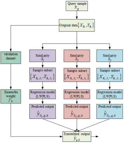
In this equation, $\gamma_k$ can be deduced from the prediction outcomes of the cross-validation dataset, with the projected result represented as $\hat{y}_{h, K}$, where h denotes the count of sub-models derived from the cross-validation dataset. The mean squared error (RMSE) corresponding to each similarity measure $S_K$ is laid out in Eq. (22). Following this, the weight $\gamma_k$ tied to the prediction outcomes for each similarity measure $S_K$ can be discerned as shown in Eq. (23). Conclusively, local online models crafted via these three similarity measures are weighted for output, with the procedural flow chart of the enhanced model depicted in Figure 1.
$R M S E_K=\sqrt{\frac{1}{h} \sum_{i=1}^h\left(y_h-\hat{y}_{h, K}\right)^2}$ (22)
$\gamma_k=e^{-\left(R M S E_K\,\right)\,^2} / \sum_{i=1}^K e^{-\left(R M S E_i\,\right)\,^2}$ (23)
Figure 1. Schematic representation of multi-similarity metric-driven JITL
Figure 2. Illustration of dataset division through moving windows
Figure 3. Schematic of the ensemble learning-based weighting strategy for moving windows
2.3 Dynamic partitioning of datasets with moving windows
The imperative nature of selecting apt sample sets in immediate learning strategies is well-recognized. However, extracting sample sets from exhaustive historical data imposes an excessive computational load. In the study of the fermentation process of Saccharomyces cerevisiae, a continuously fluctuating biochemical reaction is observed. Due to the similarity in data attributes from consecutive time intervals, an MW approach is advocated for the preliminary selection of analogous samples.
MW, characterized as an adaptive modeling technique, operates on the basis of sampling time. Historical samples are systematically divided into subsequent moving window modules, ensuring the presence of data with congruent attributes within individual windows. With the progression of time, updates to the dataset are made by discarding aged samples and introducing newer ones (as illustrated in Figure 2).
As demonstrated in Figure 2, let the window length be denoted by L. Upon the arrival of a query sample, it is positioned at the extreme right of the window. The first window's data matrix is represented as $\left\{X_{B_1}, Y_{B_1}\right\}$. With each successive movement, the window shifts one unit rightward along the time axis, marking the input and output datasets as $\left\{X_{B_2}, Y_{B_2}\right\}$. This action is reiterated until the query sample aligns with the window's leftmost end.
A pivotal aspect of the moving window technique is the determination of an optimal window length, L. Overly extensive windows risk encompassing redundant samples, thereby amplifying computational complexity. On the contrary, extremely narrow windows may not aptly represent process variability. Sadly, no universal method exists for ascertaining the perfect window size, making repetitive experimentation a standard approach to derive a suitable value.
Simulations revealed a notable observation: minor movements of the window often led to significant similarities in data across neighboring windows. Such a scenario precipitates the construction of sub-models with excessive resemblances, inadvertently increasing computational intricacies and potentially impairing predictive accuracy. To maintain diversity within sub-datasets, the concept of cumulative similarity threshold was integrated, as delineated in Eq. (24) [19].
$\eta_k=\frac{\sum_{i=1}^L \,S_{q i, s u b(k+1)}}{\sum_{i=1}^L \,S_{q i, s u b(k)}}$ (24)
where, $\eta_k$ epitomizes the proportion of the cumulative similarity of group k+1's sub-dataset to that of group k. L signifies the count of sampling points encompassed within the window. If $\eta_k \in[1-\varepsilon, 1+\varepsilon]$, subset k+1 is negated and exempted from modeling. Conversely, a value indicates the prevalent diversity within the windowed sub-dataset. Cumulative similarity, $\eta_k$, was ascertained utilizing the cross-validation method, represented by ε=0.5.
Significantly, the algorithm's foundation, represented by the moving window, only employs the similarity measure $S_1$ as the exclusive screening criterion for moving window selection in this research.
2.3.1 Ensemble learning application to moving windows
For enhanced prediction accuracy, an ensemble learning strategy was incorporated to amalgamate the results from each window's data output. This fusion process is achieved using a weighted average method, expressed in Eq. (25).
$H(x)=\sum_{i=1}^T \rho_i h_i(x)$ (25)
In the above equation, $\rho_i$ stands for the weightage of the base learner $h_i(x)$ within the ith moving window, and T represents the quantity of moving windows post-filtration. Weight calculations were based on the moving window's screening criteria mentioned earlier. By leveraging the weighted averaging algorithm, improvements in learner generalization and predictive precision were observed. A comprehensive flow chart detailing the construction of a moving window model via ensemble learning is provided in Figure 3.
Figure 4. Schematic representation of the EK-MW-LWPLS algorithm modeling
2.4 Auxiliary variable selection through k-nearest neighbor mutual information
The fermentation process of Pichia pastoris is delineated as a multi-phasic operation. Within its distinct stages, auxiliary variables exert varied influences upon the principal parameters. In specific fermentation phases, certain environmental variables are necessitated to be meticulously adjusted and sustained at designated values. Consequently, these variables remain unamenable to localized modeling. A challenge arises when JITL indiscriminately employs auxiliary variables for both local and global modeling, inadvertently compromising model precision.
In light of the aforementioned concerns, a strategy for pre-selecting auxiliary variables for sample data, defined by the moving window's range, was devised. It should be underscored that this approach abstains from filtering the auxiliary variables for each data subset derived from the moving window. As the query sample is presented, the auxiliary variables spanning the entire sample data traversed by the moving window are mandated to undergo filtering through the application of the k-MI algorithm [20].
Shannon's [21] proposition of mutual information serves as a metric quantifying the interrelation between variables. Mutual information is emblematic of the shared data between the random variables x and y. A pronounced correlation between two random variables is directly proportional to an augmented mutual information. The computation of mutual information is depicted in Eq. (26).
$I(x, y)=\iint p(x, y) \lg \frac{p(x, y)}{p(x) p(y)} d x d y$ (26)
In the equation, p(x) and p(y) represent the marginal probability distributions of the random variables x and y, respectively, whilst p(x, y) symbolizes the joint probability distribution intertwining the two random variables. Acquiring the probability distributions amidst the auxiliary variables in Pichia pastoris's fermentation process is recognized as an intricate task. Employing the k-MI algorithm has been observed to efficiently mitigate the computational strain. Furthermore, the algorithm's capability to curtail the count of auxiliary variables markedly enhances the model's reaction velocity. The k-MI algorithm's computation is elucidated in Eq. (27).
$I(x, y)=\Psi(k)-1 / k-\left\langle\Psi\left(n_x\right)+\Psi\left(n_y\right)\right\rangle+\Psi(N)$ (27)
The EK-MW-LWPLS algorithm's modeling flow is graphically presented in Figure 4.
For a lucid understanding of the soft sensor model's construction, the modeling strategy is elucidated through the subsequent sequence:
Step 1: Data spanning multiple batches are amassed, consequent to which a comprehensive database is established. Thereafter, an ordering of the data based on the temporal aspect of sampling is executed.
Step 2: The length of the moving window is designated as L, leading to the calculation of the cumulative span across which the moving window is to traverse. Within the circumscribed local range, the k-MI algorithm is deployed for the discerning selection of auxiliary variables.
Step 3: A systematic sliding of the moving window, commencing from the leftmost bound and concluding when the query sample aligns with the window's left extremity, culminates in the generation of N distinct sub-datasets.
Step 4: Three distinct methodologies for gauging similarity are explored, of which the similarity measure, S1, is employed for the computation of the cumulative similarity threshold. This step results in the elimination of superfluous moving windows.
Step 5: A disaggregated approach is adopted; wherein disparate similarity measures undergo individual training sessions tailored to the sub-models under the purview of the MW-LWPLS algorithm.
Step 6: Variegated moving windows facilitate the creation of sub-models. Subsequently, predictions derived from these are amalgamated via a weighted average, culminating in the final output.
4.1 Procedural overview of Pichia pastoris fermentation
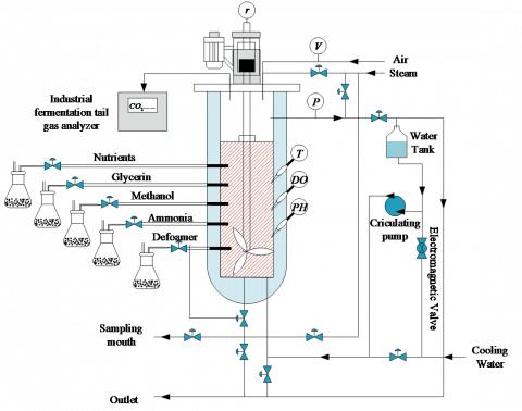
Employing the fermentation process of Pichia pastori as the focal point, the strain Pichia pastoris GS115, MutS His+ was chosen for the experimental trials. The pilot platform, furnished by Yangzhong Jiaocheng Biotechnology Research Co., Ltd, served as the venue for the completion of the fermentation process, utilizing the A103-500L model of the fermentation tank. A visual representation of the Pichia pastoris fermentation process can be observed in Figure 5.
Figure 5. Schematic of the Pichia pastoris fermentation process
5.1 Determination of auxiliary variables
Upon examination of the Pichia pastoris fermentation mechanism, both cell concentration X and product concentration S were identified as primary variables in the process. In this context, 16 environmental variables, which can be directly measured, were elected as auxiliary variables, delineated in Table 1.
Table 1. 16 Directly measurable environmental variables
|
Variable Name |
Identifier |
Variable Name |
Identifier |
|
Dissolved oxygen concentration |
DO |
Flow of air |
l |
|
Exhaust CO2 concentration |
$\eta_{\mathrm{CO}_2}$ |
Flow rate of condensate |
fw |
|
pH of fermentation broth |
pH |
Flow acceleration rate of ammonia |
fa |
|
Fermentation temperature |
T |
Flow acceleration rate of inorganic salts |
fb |
|
Pressure in the fermenter |
P |
Flow acceleration rate of glucose |
fc |
|
Volume of fermentation broth |
V |
Flow acceleration rate of peptones |
fd |
|
Fermentation time |
t |
Flow acceleration rate of glycerine |
fe |
|
Motor stirring speed |
r |
Flow acceleration rate of methanol |
ff |
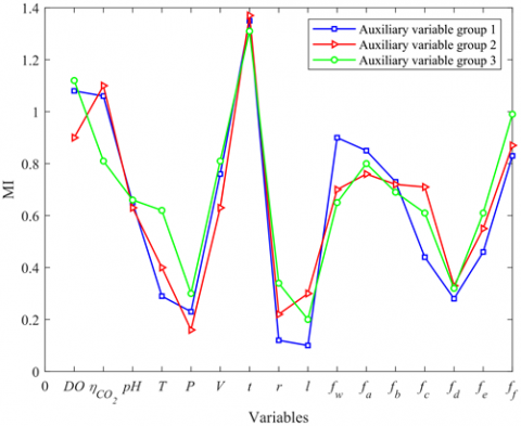
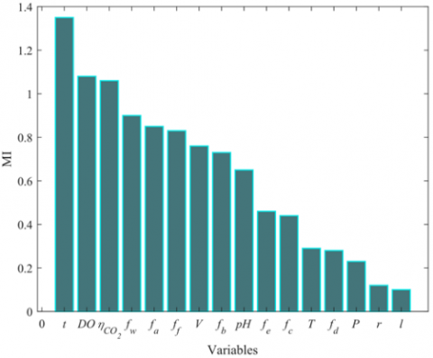
Utilizing the k-MI algorithm, a screening of auxiliary variables was conducted. Subsequently, mutual information between the environmental variables and cell concentration was calculated and sequenced based on magnitude, as depicted in Figure 6. Figure 6(a) presents the mutual information between environmental variables and cell concentrations, corresponding to query variables across three distinct stages. Meanwhile, Figure 6(b) portrays the mutual information between the environmental variables and cell concentration related to a specific stage's query variables, methodically sequenced by magnitude. In this study, the six paramount environmental variables, in terms of correlation, were chosen to formulate the soft sensor predictive models. A given stage's query variable aligns with a cell concentration's predictive model, exemplified in Eq. (28).
$\phi(X)=f\left(t, \eta_{\mathrm{Co}_2}, f_w, f_a, f_f\right)$ (28)
(a)
(b)
Figure 6. Mutual information association between environmental variables and cell concentrations within moving windows across diverse query variables, and arrangement of mutual information between environmental variables and cell concentrations for singular query variable
5.2 Ascertainment of moving window length
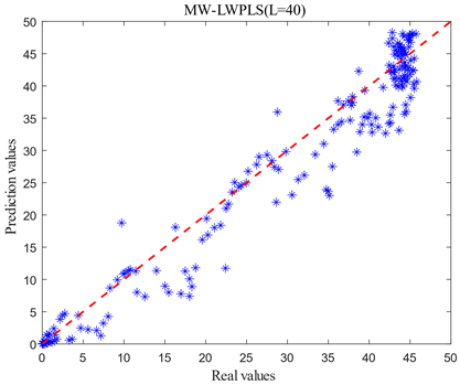
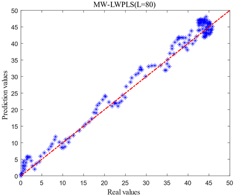
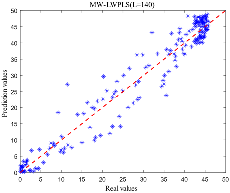
For optimizing computational efforts and enhancing modeling efficiency, it is imperative that the length of moving windows remains minimal while safeguarding model accuracy. Given the existence of nine data batches within the database, it was observed that excessively short or long moving window lengths directly influenced predictive outcomes. Under the stipulated condition L∈[20,140], the MW-LWPLS model's predictive accuracy was evaluated at intervals of 20 sampling points. The corresponding predictive results are presented in Figure 7.
(a)
(b)
(c)
(d)
(e)
(f)
Figure 7. Comparison of prediction models with different window lengths
Table 2. Performance indicators of the MW-LWPLS model for predicting cell concentration at different window lengths
|
MW-LWPLS |
L=40 |
L=60 |
L=80 |
L=100 |
L=120 |
L=140 |
|
RMSE |
4.2555 |
3.0126 |
2.2865 |
2.8173 |
3.1712 |
3.9526 |
|
R2 |
0.9295 |
0.9647 |
0.9796 |
0.9691 |
0.9608 |
0.9392 |
As shown in Figure 7, when L=40 and L=140, the actual and predicted values of cell concentration are significantly shifted, and dispersion was large. When L=60 and L=120, the prediction of pre-fermentation and smooth period was more satisfactory, but the error of the exponential growth period of fermentation was larger. If there is a large error in prediction during the exponential growth period of fermentation, it will lead to an inability to replenish the raw material in time for the fermentation process, thus making the fermentation less effective than expected and affecting the yield. When L=80 and L=100, the dispersion of the prediction results becomes significantly smaller. To further determine the length of the moving window L, the root means square error (RMSE) and the coefficient of determination (R2) are used as criteria for judging the model, as shown in Table 2.
Table 2 shows that RMSE decreases and R2 increases as the length of L increases from 40 to 80. As the L length increases from 80 to 140, the RMSE increases, and the R2 decreases. Therefore, the optimal window length of around 80 can be determined and applied to the subsequent soft sensor model.
5.3 Simulation results and analysis of the Ek-MW-MSLWPLS model
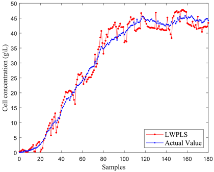
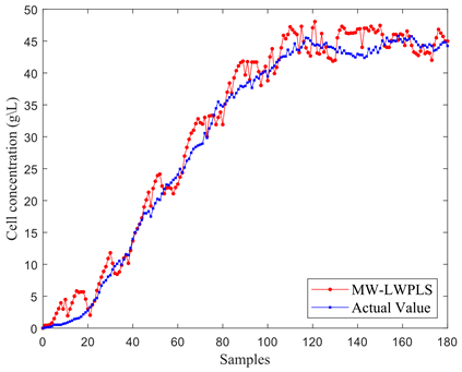
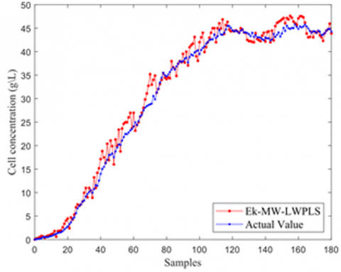
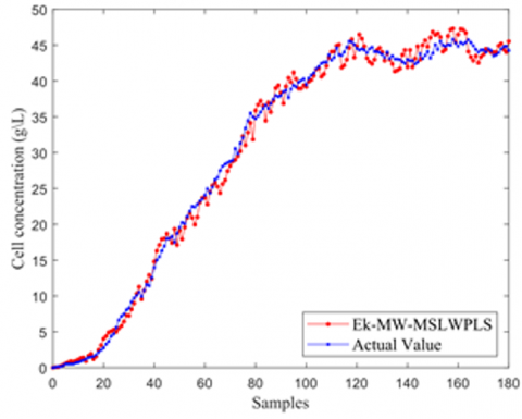
Upon the ascertainment of the optimal window length, the LWPLS model, MW-LWPLS model, Ek-MW-LWPLS model, and Ek-MW-MSLWPLS model were constructed to assess the relative efficacy of the Ek-MW-MSLWPLS algorithm. Predictive results for cell concentration across these models are illustrated in Figure 8.
(a)
(b)
(c)
(d)
Figure 8. Depiction of cell concentration predictive curves across four model types
In Figure 8(a), notable deviations between the predictive cell concentration curve and the actual curve were observed. Figure 8(b) highlights how, upon incorporating a moving window for cell concentration predictions, a reduction in overall bias was achieved, though certain phases still manifested pronounced errors. Figure 8(c) exhibits a method where both local auxiliary variable selection and an integrated algorithm for moving window optimization were integrated into the model from Figure 8(b). This integration led to marked enhancements in predictive accuracy, albeit with heightened fluctuations and dispersed individual predictive points. The implementation of a multi-similarity measurement-driven model combined with an integrated output approach in Figure 8(d) revealed superior predictive accuracy, with curves aligning more closely.
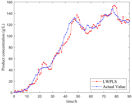
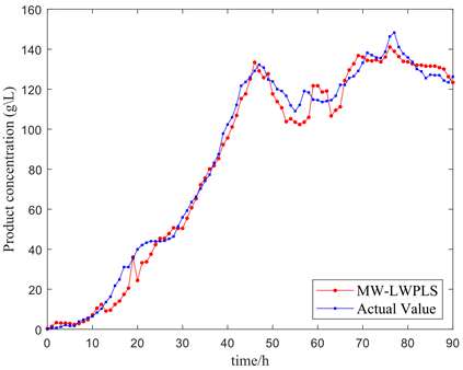
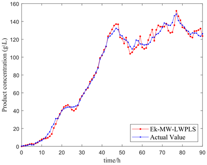
Further validation of the algorithm's feasibility entailed employing the model to predict the product concentration of Pichia pastoris, illustrated in Figure 9. The integration of the moving window ostensibly refined the sample search scope, subsequently bolstering the efficacy of the local model compared to a broader search. A comparison between Figures 9(a) and 9(b) highlighted the moving window's instrumental role in bolstering the model's curve tracking capacity. Yet, a sharp alteration in the actual curve revealed a deficiency in the model's tracking proficiency, as evidenced in Figure 9(c). Nevertheless, Figure 9(d) demonstrates that the introduction of multiple similarity metrics significantly mitigated this issue.
(a)
(b)
(c)
(d)
Figure 9. Four model predictive curves for cell concentration
(a)
(b)
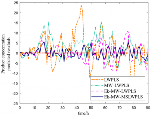
Figure 10. Predictive residual curve comparisons for cell and product concentrations
To facilitate a comprehensive comparison across the four models, evaluative metrics, namely the root mean square error (RMSE), coefficient of determination (R2), mean relative error (MRE), and maximum absolute error (MAX), were employed. Table 3 presents these results, signifying that the Ek-MW-MSLWPLS model's RMSE, MRE, and MAX were markedly inferior to those of the other models, while its R2 approached unity, indicating a superior performance of the Ek-MW-MSLWPLS soft sensor model. For a more tangible comparison of the predictive capabilities of the four models, predictive residuals for both bacterial and product concentrations are showcased in Figure 10. A discernible superiority of the Ek-MW-MSLWPLS soft sensor model over its counterparts is evident.
Table 3. Comparative analysis of cell and product concentration predictive errors across models
|
Model |
Cell Concentration |
Product Concentration |
||||
|
RMSE |
R2 |
RMSE |
R2 |
MRE |
MAX |
|
|
LWPLS |
2.3429 |
0.9786 |
7.4669 |
0.9767 |
0.1890 |
23.6771 |
|
MW-LWPLS |
2.2865 |
0.9796 |
5.8894 |
0.9855 |
0.1687 |
15.5456 |
|
Ek-MW-LWPLS |
1.7118 |
0.9886 |
4.2426 |
0.9925 |
0.0894 |
10.7623 |
|
Ek-MW-MSLWPLS |
1.2494 |
0.9939 |
2.2875 |
0.9978 |
0.0877 |
5.5007 |
The fermentation process involving Pichia pastoris has been characterized by its temporal variability, inherent delay, and non-linearity. In situations where environmental conditions undergo alterations, offline models have been observed to falter. To address these challenges, the Ek-MW-MSLWPLS soft sensor model was introduced, offering an online solution. Data subsets were delineated through moving windows, and, within these data subsets, explanatory variables underwent filtration via the k-MI algorithm. Local modeling was driven by a multi-similarity measurement, promoting timely learning. As a culminating step, dual ensemble learning facilitated the amalgamation of all models present in the sub-datasets. Based on the experimental outcomes, it was deduced that the Ek-MW-MSLWPLS model possesses the capability to predict cell and product concentrations online with precision.
[1] Kalinina, A.N., Borshchevskaya, L.N., Gordeeva, T.L., Sineoky, S. (2019). Comparison of xylanases of various origin obtained in the expression system of Pichia pastoris: Gene expression, biochemical characteristics, and biotechnological potential. Applied Biochemistry and Microbiology, 55: 733-740. https://doi.org/10.1134/S0003683819070044
[2] Abdulrachman, D., Thongkred, P., Kocharin, K., Nakpathom, M., Somboon, B., Narumol, N., Chantasingh, D. (2017). Heterologous expression of Aspergillus aculeatus endo-polygalacturonase in Pichia pastoris by high cell density fermentation and its application in textile scouring. BMC Biotechnology, 17(1): 1-9. https://doi.org/10.1186/s12896-017-0334-9
[3] Mohanty, S., Khasa, Y.P. (2021). Nitrogen supplementation ameliorates product quality and quantity during high cell density bioreactor studies of Pichia pastoris: A case study with proteolysis prone streptokinase. International Journal of Biological Macromolecules, 180: 760-770. https://doi.org/10.1016/j.ijbiomac.2021.03.021
[4] Ahmad, M., Hirz, M., Pichler, H., Schwab, H. (2014). Protein expression in Pichia pastoris: Recent achievements and perspectives for heterologous protein production. Applied Microbiology and Biotechnology, 98: 5301-5317. https://doi.org/10.1007/s00253-014-5732-5
[5] Martens, T. (2021). Urgent cardiac surgery and COVID-19 infection: Uncharted territory: Reply. The Annals of Thoracic Surgery, 111(5): 1735. https://doi.org/10.1016/j.athoracsur.2020.09.007
[6] Zhang, Y., Wang, J., Liu, X. (2021). Selective quenching detection of proteinase K by croconaine based organic sensor. World Scientific Research Journal, 7(4): 472-479. https://doi.org/10.6911/WSRJ.202104_7(4).0058
[7] Wang, B., He, M., Wang, X., Tang, H., Zhu, X. (2022). A multi-model predictive control method for the Pichia pastoris fermentation process based on relative error weighting algorithm. Alexandria Engineering Journal, 61(12): 9649-9660. https://doi.org/10.1016/j.aej.2022.03.004
[8] Zhu, X., Rehman, K.U., Wang, B., Shahzad, M. (2020). Modern soft-sensing modeling methods for fermentation processes. Sensors, 20(6): 1771. https://doi.org/10.3390/s20061771
[9] Huang, L., Wang, Z., Ji, X. (2016). LS-SVM generalized predictive control based on PSO and its application of fermentation control. Proceedings of the 2015 Chinese Intelligent Systems Conference, Xi’an, China, Volume 1, pp. 605-613. https://doi.org/10.1007/978-3-662-48386-2
[10] Dave, N., Varadavenkatesan, T., Selvaraj, R., Vinayagam, R. (2021). Modelling of fermentative bioethanol production from indigenous Ulva prolifera biomass by Saccharomyces cerevisiae NFCCI1248 using an integrated ANN-GA approach. Science of The Total Environment, 791: 148429. https://doi.org/10.1016/j.scitotenv.2021.148429
[11] Yang, C., Zhao, Y., An, T., Liu, Z., Jiang, Y., Li, Y., Dong, C. (2021). Quantitative prediction and visualization of key physical and chemical components in black tea fermentation using hyperspectral imaging. LWT, 141: 110975. https://doi.org/10.1016/j.lwt.2021.110975
[12] Ren, M., Song, Y., Chu, W. (2019). An improved locally weighted PLS based on particle swarm optimization for industrial soft sensor modelling. Sensors, 19(19): 4099. https://doi.org/10.3390/s19194099
[13] Yamada, N., Kaneko, H. (2021). Adaptive soft sensor ensemble for selecting both process variables and dynamics for multiple process states. Chemometrics and Intelligent Laboratory Systems, 219: 104443. https://doi.org/10.1016/j.chemolab.2021.104443
[14] Yuan, X., Ge, Z., Song, Z. (2016). Spatio-temporal adaptive soft sensor for nonlinear time-varying and variable drifting processes based on moving window LWPLS and time difference model. Asia-Pacific Journal of Chemical Engineering, 11(2): 209-219. https://doi.org/10.1002/apj.1957
[15] Yuan, X., Zhou, J., Wang, Y., Yang, C. (2018). Multi-similarity measurement driven ensemble just-in-time learning for soft sensing of industrial processes. Journal of Chemometrics, 32(9): e3040. https://doi.org/10.1002/cem.3040
[16] Liu, Y., Gao, Z., Li, P., Wang, H. (2012). Just-in-time kernel learning with adaptive parameter selection for soft sensor modeling of batch processes. Industrial & Engineering Chemistry Research, 51(11): 4313-4327. https://doi.org/10.1021/ie201650u
[17] Cheng, C., Chiu, M.S. (2004). A new data-based methodology for nonlinear process modelling. Chemical Engineering Science, 59(13): 2801-2810. https://doi.org/10.1016/j.ces.2004.04.020
[18] Yuan, X., Huang, B., Ge, Z., Song, Z. (2016). Double locally weighted principal component regression for soft sensor with sample selection under supervised latent structure. Chemometrics and Intelligent Laboratory Systems, 153: 116-125. https://doi.org/10.1016/j.chemolab.2016.02.014
[19] Zhu, X., Cai, K., Wang, B., Rehman, K.U. (2021). A dynamic soft sensor modeling method based on MW-ELWPLS in marine alkaline protease fermentation process. Preparative Biochemistry & Biotechnology, 51(5): 430-439. https://doi.org/10.1080/10826068.2020.1827428
[20] Kraskov, A., Stögbauer, H., Grassberger, P. (2004). Estimating mutual information. Physical Review E, 69(6): 066138. https://doi.org/10.1103/PhysRevE.69.066138
[21] Shannon, C.E. (1949). Communication theory of secrecy systems. The Bell System Technical Journal, 28(4): 656-715. https://doi.org/10.1002/j.1538-7305.1949.tb00928.x