Carlos E.R.B. Barateiro*![]() | Mauricio Casado
| Mauricio Casado![]() | Claudio Makarovsky
| Claudio Makarovsky![]() | Jose R. de Farias Filho
| Jose R. de Farias Filho![]()
© 2023 IIETA. This article is published by IIETA and is licensed under the CC BY 4.0 license (http://creativecommons.org/licenses/by/4.0/).
OPEN ACCESS
Volumes produced measurement is essential for royalties and governments participation calculating at crude oil and natural gas production fields concession contracts. This remuneration is a common model and for that, so rules and regulations are issued that must be followed by operators, with very clear procedures to be followed. However, these specifications allow a certain degree of choice among the available technological alternatives, and it is up to the operator to ensure that they meet the specifications. And here there is a difficult decision to be made: should the choice focus only on the cost of CAPEX and OPEX of the technological alternative? Metering stations operating cost (OPEX) and investment cost (CAPEX) varies depending on the measurement technology chosen. But the systems uncertainty also depends on this choice and consequently, directly affects the business risk. Thus, the objective of this work is to analyze these variables, which must be considered in the decision making, starting from a revamp feasibility study of the export gas measurement systems for two practically identical offshore platforms. In the first was considered orifice plate element and for second, the use of ultrasonic flow technology. It was possible to analyze the variation of the total cost of ownership (TCO) for three years operation and compare it with the variation of the involved risk, noting that there is a clear prevalence of the second in relation to the first. And therefore, this analysis must be considered in the decision of the projects of the measurement stations.
flow measurement, business risk, total cost of ownership
The oil and natural gas market is extremely regulated because there are many interests involved. Extraction from natural reserves involves significant investments that often cannot be borne directly by federal governments. And so, several models were developed for granting the right of production to third parties (operators) [1].
The concession and production sharing are legal-fiscal regimes for oil and gas exploration. The main difference between them is the degree of State interference in operations and how the ownership of hydrocarbons is appropriated. Typically, the State does not take part in the operations, but regulates, supervisory them and take taxation, royalties, and specific contributions [2].
Regardless of the type of contract specified, the basis is the correct measurement of extracted volumes [3]. It is through this measurement that the appropriate remuneration can be made. So, States, in their role of regulating exploration activities, specify the processes and procedures to be adopted to ensure complete and accurate results [4].
In these regulations there is flexibility in the choice of solutions to be used by operators. It is possible to mention, for example for natural gas, the measurement alternatives based on differential elements, ultrasonic, Coriolis effect, V-cone, positive displacement, and turbines, which are normally recommended [5]. Each of these technologies has different measurement principles, application ranges, installation and operation criteria, influence of process conditions and therefore the expected uncertainties are not the same. In this way, the regulations specify maximum limits that must be met by operators, and it is up to them to define the most appropriate technology.
And here is the focus of this article: How to make this choice considering, on the one hand, the degree of risk inherent to the volumes produced and the measurement uncertainty and, on the other, the systems operating costs (OPEX) and the implementation investments (CAPEX) necessary for the metering stations?
To support the correct choice and allow an analysis based on quantitative aspects, two identical oil and natural gas production platforms located in very close production fields were chosen. Both have a production capacity of 304.571 Nm3/h and in the period from May 2019 to April 2022, the production was 206,945 and 192,441 Mm3/mth, respectively for the first and second production units [6].
The operating conditions are identical, and the analysis was considered that the first unit would maintain the system for measuring the flow of exported gas using an orifice plate and the second would operate using an ultrasonic meter, both in 12" lines.
Thus, it was possible to make simulations for the CAPEX and OPEX of the two stations, and from the expected uncertainties, to assess the risk in the determination of the production valuation. The variance in total cost of ownership costs and associated risks are a good parameter for evaluating the alternative to be chosen.
There are several approved technologies for these measurements. As mentioned, there are differential elements, ultrasonic, Coriolis effect, V-cone, positive displacement, and turbines. The gas produced ("exported") in offshore production units typically operates under high pressures, large volumes, and medium to large diameter lines. The flow is relatively stable with low presence of liquid phases (performed after treatment). Under these conditions, ultrasonic measurement presents itself as an interesting alternative, but several projects still use traditional constraint-based meters (orifice plates). And there are reasons for these choices with ancient technologies. Initially we need to understand how both technologies operate and their main requirements.
2.1 Orifice plate technology
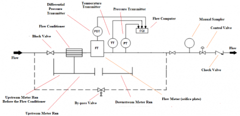
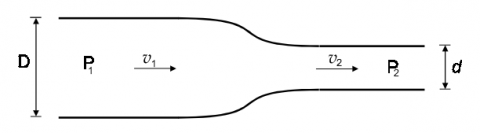
Figure 1 shows the schematic of a station for measuring natural gas using a line restriction device (orifice plate). With this, the ISO5167 standard [7] is normally used, which presents a fundamental equation for obtaining instantaneous flow by the Bernoulli Equation. This equation represents energy conservation for a fluid element and its application can best be visualized in a tube with a circular cross section that is reduced in diameter as it descends in the horizontal direction, as shown in Figure 2.
Figure 1. Natural gas metering station using a restriction device (orifice plate)
Figure 2. Flow in horizontal tube with diameter reduction
The general equation for measuring the mass flow rate used by the ISO5167 standard [7] is:
$Q_m=\frac{C_d}{\sqrt{1-\beta^4}} \varepsilon \frac{\pi}{4} d^2 \sqrt{2 \Delta P \rho_1}$ (1)
where, β=d/D with D is upstream diameter (m) and d is orifice or device throat diameter (m); ∆P=P1–P2 (Pa) with P1 is upstream pressure and P2 is downstream pressure; ρ2=ρ2 (there is no change on density upstream and downstream) and Qm is mass flow rate along the pipe (kg/s).
It is worth considering that from the equation of real gases:
$\rho_2=\rho_1=\frac{\mathrm{P}_{2 .} \cdot(\mathrm{MM})}{\mathrm{Z.} \mathrm{R.} \mathrm{T}_2}=\frac{\mathrm{P}_{1 .} \cdot(\mathrm{MM})}{\mathrm{Z.} \mathrm{R.} \mathrm{T}_1}$ (2)
With MM is gas molecular mass, R is universal constant of perfect gases (8,314462618 J mol-1 K-1), T is flowing temperature and Z is compressibility factor (depends on pressure and temperature).
The Eq. (1) is derived in part from further analysis of complex theory, but it mainly comes from experimental research done over the years and presented in various publications. What is interesting about the ISO5167 [7] standard is that it condenses all experimental research and gives it in a simple and practical way. This adaptation resulting from the experiments introduced two additional factors: Expansion Factor (ε) and Discharge Coefficient (Cd).
The Expansion Factor (dimensionless) is used to account for the fluid's compressibility, which differentiates a real fluid from a perfect gas. The numerical values of ε for orifice plates given in ISO5167-2 [7] are based on experimentally determined data. For nozzles and Venturi tubes, they are based on the general thermodynamic energy equation. For steam and gases (compressible fluids) ε<1. It is calculated with different formulas depending on device geometry. For example, for an orifice plate, ISO5167-2 gives the following formula:
$\epsilon=1-\left(0.351+0.256 \beta^4+0.93 \beta^8\right)\left[1-\left(\frac{P_2}{P_1}\right)^{1 / k}\right]$ (3)
where, k is the isentropic exponent, a property of the fluid that depends on the pressure and temperature of the fluid. It is related to the adiabatic expansion of the fluid in the orifice.
The discharge coefficient (dimensionless), set to a flow of incompressible fluid, relates the actual flow rate to the theoretical flow rate through a device. It is related to turbulent flow and the restriction that devices place on the flow. ISO5167-2 [7] provides the following formula for an orifice gauge with flange taps, diameter ratio β=d/D between 0.1 and 0.75 and:
$\begin{gathered}C_d=0.5961+0.0261 \beta^2-0,216 \beta^8+0.000521\left(\frac{10^6 \beta}{R e_D}\right)^{0.7}+(0.0188+0.0063 A) \beta^{3,5}\left(\frac{10^6}{R e_D}\right)^{0.3} \\ +\left(0.043+0.080 e^{-10 L_1}-0.123 e^{-7 L_1}\right) \cdot(1-0.11 A) \frac{\beta^4}{1-\beta^4} -0.031\left(M_2-0.8 M_2^{1.1}\right) \beta^{1.3}\end{gathered}$ (4)
where, e is the plate thickness, L1 and L2 dimensions related to the pressure taps, and M2 is the quotient of the distance of the downstream tapping from the downstream face of the plate and the dam height.
ReD is the Reynolds number calculated with respect to D defined as:
$R e_D=\frac{\rho_1 \ v_1 \ D}{\mu_1}$ (5)
where, v1 is the upstream velocity (m/s) and μ1 is the fluid dynamic viscosity (Pa.s). Viscosity is a fluid property that depends on composition, pressure, and temperature.
The Eq. (3) for discharge coefficient is named Reader-Harris/Gallagher Equation.
As noted, pressure measurement is essential in the process of obtaining the corrected flow and its value must be in absolute scale for gas measurement stations. The pressure value directly affects the density, expansion factor and discharge coefficient by the Reynolds number. With the use of pressure gauge transmitters, it is necessary to parameterize the local atmospheric pressure value in the flow computer [8].
With this technology, its necessary to keep calibrated or with some degree of meteorological control:
·Pressure transmitters.
·Differential Pressure Transmitters.
·Temperature Transmitters.
·Flow Computer.
·Orifice Plate.
·Downstream and Upstream Meter Run.
Then it is necessary to consider the following sources of uncertainty:
·Temperature Measurement.
·Static Pressure Measurement.
·Differential Pressure Measurement Across the Orifice.
·Specific Mass Calculation.
·Pipe Diameter Measurement.
·Orifice Diameter Measurement.
·Expansion Factor Calculation.
·Discharge Coefficient Calculation.
·Flow Calculation (flow computer to obtain the flow at reference conditions).
2.2 Ultrasonic technology
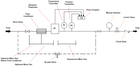
Figure 3 shows the schematic of a station for measuring natural gas using an ultrasonic flow meter. With this, the ISO 17089 standard [9] is normally used, which presents a fundamental equation for obtaining instantaneous flow by fluid continuity equation.
Figure 3. Natural gas metering station using an ultrasonic flowmeter
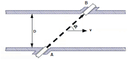
Multi-path ultrasonic meters are typically used for gas custody transfer and fiscal measurement to calculate gas flow rate from velocity measurements made over a pipe’s cross-section. This is accomplished using the following process (Figure 4) [10]:
·Transducer pairs are installed in a meter body and used to make transit time measurements of ultrasonic pulses, which each transducer transmits and receives. Pulses shot in the downstream direction are accelerated, while those shot upstream are decelerated by the gas flow.
Velocities are calculated for each transducer pair, or path, from the measured transit time difference between pulses shot in the up- and down-stream directions.
·Multiple path velocities are averaged into the bulk velocity using a weighting scheme that depends on the path’s location in the pipe cross-section for which velocity is “sampled”.
·Bulk velocity is multiplied by the meter body’s cross-sectional area to calculate uncorrected flow rate.
Figure 4. Natural gas metering station using a ultrasonic flowmeter
Velocity measurements are made along multiple paths using transducer pairs arrayed in a known position in the meter body. Since the “absolute digital travel time measurement method” is employed (firing pulses in rapid succession in opposite directions across the same flight path in the pipe), fluctuations in pressure, temperature and gas composition do not affect velocity measurement due to the nearly instantaneous sonic pulse emissions by individual transducer pairs. The flow measurement is then obtained from the transit time upstream (Eq. (6)), transit time downstream (Eq. (7)) and instantaneous velocity (Eq. (8)). The flow rate Q results from multiplying the weighted mean flow velocity (each pair of sensors) by the pipe diameter (Eq. (9)).
$t_U=\frac{L}{c-v. \cos \vartheta}$ (6)
$t_D=\frac{L}{c+v. \cos \vartheta}$ (7)
$v=\frac{L}{2. \cos \vartheta} \cdot\left(\frac{1}{t_D}-\frac{1}{t_U}\right)$ (8)
$Q=A. \bar{v}=\mathrm{A.}\left(w_1 v_1+w_2 v_2+\ldots+w_n v_n\right)$ (9)
where, tU is the transit time upstream (s), tD is transit time downstream (s), L is path length (m), c is sound velocity (m/s), ϑ is path angle, v is path velocity (m/s), A is tubing cross-sectional area (m2) and w is the weighting factor (dimensionless).
With this technology, its necessary to keep calibrated or with some degree of meteorological control:
·Pressure transmitters.
·Temperature Transmitters.
·Flowmeter.
·Flow Computer.
·Downstream and Upstream Meter Run.
Then it is necessary to consider the following sources of uncertainty:
·Temperature Measurement.
·Static Pressure Measurement.
·Pipe Diameter Measurement.
·Flowmeter Measurement.
·Flow Calculation (flow computer to obtain the flow at reference conditions).
2.3 Metering station requirements
The process of measuring volumes of oil and natural gas involves many processes in addition to primary (flow), secondary (pressure and temperature) and tertiary (flow computers) measurements. The guarantee of the quality of the results is also a function of many steps that constitute the metrological control [5]. It can be mentioned:
·Chemical and physical analysis of fluids.
·Data, Alarm & Event Logs Control.
·Uncertainty Calculation and Control.
·Audit and Traceability.
·Maintenance and Inspection Routines.
·Calibration and Proving.
Fluid characteristics need to be monitored because are used to obtain corrected flow or volume values either through the direct parameters in the compensation equations (algorithms) or indirectly because they affect direct parameters.
Control of data, alarms and events is essential for validating processes and allowing traceability of results. Monitoring uncertainties is equally important to verify that measurements are occurring within acceptable error standards. Audits are primarily intended to verify whether the routines and parameters being used are in accordance with what was expected. Maintenance and periodic inspections are intended to ensure that equipment continues to operate in accordance with good industry practices and mainly to analyze the impacts of fluid flow on this equipment.
Proving is the process to check a flow meter against a reference device to evaluate the difference between both. After a several runs are taking note of the differences in the measure value of each device (operational and reference) and with that it is possible to calculate the factor called "K" – this “K” factor is used to calibrate the operational meter. Calibration is whatever is necessary to adjust the meter to match the reference device ensuring accurate measurement performance [11].
Measurement regulations define the maximum calibration frequency of primary and secondary meters according to equipment type, application, and technology [4]. Table 1 presents the main periodicities defined for the Brazilian gas market (focus of this work).
Mainly for fiscal and custody transfer applications, the deadlines are short. There is yet another complicating factor: many of the calibrations need to be carried out in laboratories accredited according to ISO 17025 [12] - which implies the removal of the meters from the plant, bringing costs of logistics and the service provided. Particularly, Brazil has few laboratories capable of calibrating meters for high flows and, therefore, there is a need to use laboratories in Europe and the United States.
The calibration of pressure, differential pressure and temperature gauges is relatively easy to perform in the plant itself, and as the inspection period for straight sections and orifice plates is relatively long (36 months), the orifice plate measurement technology ends up being chosen in many projects, even without having the same level of uncertainty as other more current technologies.
Table 1. Brazilian calibration and inspection frequencies
|
Metering Technology |
Application (months) |
||
|
Fiscal |
Allocation |
Custody Transfer |
|
|
Reference by Displacement, Rotary and Turbine |
6 |
12 |
18 |
|
Reference by Coriolis |
12 |
12 |
12 |
|
Reference by Ultrasonic |
30 |
12 |
12 |
|
Reference by Other Technology |
6 |
12 |
12 |
|
Operational by Positive Displacement, Rotary and Turbine |
3 |
6 |
18 |
|
Operational by Coriolis |
6 |
12 |
12 |
|
Operational by Ultrasonic |
6 |
12 |
12 |
|
Operational by Other Technology |
3 |
6 |
12 |
|
Temperature |
3 |
6 |
6 |
|
Pressure |
3 |
6 |
6 |
|
In-Line Chromatograph or Density Analyzer |
6 |
12 |
12 |
|
Primary Pressure Differential Element |
12 |
12 |
12 |
|
Orifice Fitting |
36 |
36 |
36 |
|
Meter Run for Primary Pressure Differential Element |
36 |
36 |
36 |
|
Meter Run for Other Technologies |
36 |
36 |
36 |
|
Manual Samplers |
12 |
12 |
12 |
Source: ANP, 2013
Typically, operators have their own or contracted teams to perform the tasks of metrological control and calibration of these simpler equipment, and they use external laboratories for activities that cannot be carried out in the plants.
Table 2. Process data
|
Process Data |
Platform A |
Platform B |
|
Metering Technology |
Orifice Plate |
Ultrasonic Flow Meter |
|
Flow Metering |
Export Gas |
Export Gas |
|
Flow Range |
30.457 to 304.571 Nm3/h |
30.57 to 304.571 Nm3/h |
|
Design Pressure/Temperature |
28000 kPag @ 93.3℃ |
28000 kPag @ 93.3℃ |
|
Density Standard Condition |
266 kg/$m^3$ |
266 kg/$m^3$ |
|
Natural Gas Molar Weight |
21.29 |
21.29 |
|
Natural Gas Viscosity at Operating Condition |
0.0318 cP |
0.0318 cP |
|
Compressibility Factor; Z |
0.771 |
0.771 |
|
Ratio Specific Heats; Cp/Cv |
1.79 |
1.79 |
|
Flanges Rating |
2500# RTJ |
2500# RTJ |
|
Line Size / Schedule |
12" / 160 |
12" / 160 |
|
Pipe Material |
API 5L-X65 PSL2 SMLS(BE) |
API 5L-X65 PSL2 SMLS(BE) |
To quantify the technology's impacts on risk and total cost of ownership, simulations were carried out in two relatively close offshore production units, whose measurement systems for the produced (exported) gas are summarized in Table 2.
Table 3 shows the natural gas production (export) at these units from May 2019 to April 2022.
Table 3. Production history
|
Date |
Production (M$m^3$) |
|
|
Platform A |
Platform B |
|
|
May/19 |
175,959 |
229,638 |
|
June/19 |
173,374 |
62,959 |
|
July/19 |
172,308 |
220,118 |
|
August/19 |
201,744 |
237,522 |
|
September/19 |
209,902 |
149,267 |
|
October/19 |
230,369 |
234,122 |
|
November/19 |
228,193 |
233,267 |
|
December/19 |
219,058 |
239,187 |
|
January/20 |
234,165 |
245,236 |
|
February/20 |
219,436 |
229,601 |
|
March/20 |
188,692 |
142,596 |
|
April/20 |
226,674 |
214,027 |
|
May/20 |
238,512 |
160,098 |
|
June/20 |
226,935 |
222,883 |
|
July/20 |
229,811 |
229,927 |
|
August/20 |
227,445 |
219,124 |
|
September/20 |
222,247 |
194,823 |
|
October/20 |
93,475 |
207,277 |
|
November/20 |
191,897 |
81,611 |
|
December/20 |
204,687 |
196,611 |
|
January/21 |
207,331 |
193,384 |
|
February/21 |
183,576 |
180,360 |
|
March/21 |
193,667 |
196,050 |
|
April/21 |
149,334 |
167,737 |
|
May/21 |
195,934 |
150,204 |
|
June/21 |
197,530 |
194,306 |
|
July/21 |
204,442 |
197,306 |
|
August/21 |
199,283 |
203,710 |
|
September/21 |
200,337 |
181,938 |
|
October/21 |
223,109 |
136,411 |
|
November/21 |
221,502 |
196,729 |
|
December/21 |
234,403 |
193,702 |
|
January/22 |
239,599 |
208,103 |
|
February/22 |
221,030 |
180,023 |
|
March/22 |
241,616 |
203,660 |
|
April/22 |
222,445 |
194,353 |
|
Average |
206,945 |
192,441 |
Based on these data it was possible to specify the measurement stations based on Figures 1 and 3 and then calculate the expected uncertainty for these stations. Table 4 shows the uncertainty assessment statement for platform A (orifice plate) and Table 5 shows the same calculation for platform B (ultrasonic). We can see that platform A will operate with a typical uncertainty of +/- 1.07% and platform B with 0.75%.
Considering the value of natural gas published monthly by the Brazilian regulatory agency, the monthly production and the expected uncertainty, Table 6 shows the risk assessment that these systems were exposed at 36 months.
Even with platform A producing 8% higher than B (206,945 against 192,441 MR\$), the exposure difference was 58% (75,582 against 47,932 MR$).
Table 4a. Uncertainty assessment for “platform A” exported gas station – Part 1
|
Process Conditions |
Symbol |
Value |
Unit |
|
Confidence level |
95 |
% |
|
|
Temperature (Base conditions) |
Tb |
20 |
℃ |
|
Pressure (Base conditions) |
Pb |
101 |
kPa(a) |
|
Pressão atmosférica: |
Pa |
100 |
kPa(a) |
|
Atmospheric pressure |
Pa |
100 |
kPa(a) |
|
Standard flow rate |
qb |
2.87E+05 |
m³/h |
|
Differential pressure |
ΔP |
33.01 |
kPa |
|
Temperature (Operational conditions) |
To |
40 |
℃ |
|
Pressure (Operational conditions) |
Po |
25100 |
kPa(g) |
Table 4b. Uncertainty assessment for “platform A” exported gas station – Part 2
|
Uncertainty Variable |
Symbol |
Value |
Standard Uncertanty |
Sensitivity Coef. |
% |
|
Orifice plate internal diameter |
d |
178.83 mm |
1.3000E-05 m |
9.1506E+02 |
0.1625 |
|
Meter run internal diameter |
D |
275.062 mm |
2.5500E-04 m |
1.0629E+02 |
0.8765 |
|
Differential pressure |
ΔP |
33.013 KPa |
1.2500E+02 Pa |
1.0180E-03 |
19.2873 |
|
Expansion coefficient |
ε |
1 |
7.7966E-06 |
6.7214E+01 |
0.0003 |
|
Discharge coefficient |
C |
0.602 |
1.7938E-03 |
1.1158E+02 |
47.7418 |
|
Density (Operational conditions) |
ρ |
245.605 kg/m³ |
1.1966E+00 kg/m³ |
1.3681E-01 |
31.9316 |
|
Expanded uncertainty (95% of confidence level, z=1.96) |
3073.32 |
m³/h |
|||
|
Standard volumetric flow rate |
6898 |
Mm³/day |
|||
|
Relative expanded uncertainty (95% of confidence level, z=1.96) |
1.07 |
% |
|||
Table 5a. Uncertainty assessment for “platform B” exported gas station – Part 1
|
Process Conditions |
Symbol |
Value |
Unit |
|
Confidence level |
- |
95 |
% |
|
Temperature (Base conditions) |
Tb |
20 |
℃ |
|
Pressure (Base conditions) |
Pb |
101.325 |
kPa(a) |
|
Atmospheric pressure |
Pa |
100 |
kPa(a) |
|
Gross flow rate |
qv |
935.6 |
m³/h |
|
Fluid velocity |
qb |
4.86 |
m/s |
|
Temperature (Operational conditions) |
To |
40 |
℃ |
|
Pressure (Operational conditions) |
Po |
25000 |
kPa(a) |
Table 5b. Uncertainty assessment for “platform B” exported gas station – Part 2
|
Uncertainty Variable |
Symbol |
Estimative |
Standard Uncertanty |
Sensitivity Coefficient |
Contribution |
|
Gross flow rate |
qv |
9.3560E+02 m³/h |
1.1695E+00 m³/h |
2.8567E+02 |
1.0606% |
|
Pressure (Operational conditions) |
Po |
2.5000E+04 KPa(a) |
6.2750E+01 KPa(a) |
1.0691E+01 |
42.7623% |
|
Temperature (Operational conditions) |
To |
4.0000E+01℃ |
1.0000E-01℃ |
8.5349E+02 |
0.6922% |
|
Compresibility Factor (Op. conditions) |
Zo |
9.9684E-01 |
2.0561E-03 |
3.3161E+05 |
44.1731% |
|
Compresibility Factor (Std. conditions) |
Zb |
8.0598E-01 |
5.0860E-04 |
2.6812E+05 |
1.7669% |
|
Expanded uncertainty (95% of confidence level, z=1.96) |
2010.67 |
m³/h |
|||
|
Standard volumetric flow rate |
6414 |
Mm³/dia |
|||
|
Relative expanded uncertainty (95% of confidence level, z=1.96) |
0.75 |
% |
|||
It remains then to carry out the evaluation of CAPEX and OPEX to implement the change. For the purposes of the analysis, the costs of hardware, software, design, and services for the construction of the stations were considered, which were obtained from a traditional manufacturer of this type of solution. For the OPEX, only the calibration costs were considered, since the others related to metrological control are independent of the type of technology. For the evaluation, the periodicities defined in the Brazilian legislation, and which are presented in Table 1 were used, as well as the costs of international flow laboratories and transport logistics. Table 7 consolidates the analysis performed.
The solution with ultrasonic has a total cost of ownership about 77% higher than that presented with the traditional solution with orifice plate.
However, there is an increase in 13.3 to 23.58 MR\$ for the total cost of ownership (TCO) against 47,932 to 75,582 MR\$ for risk. The order of magnitude is extremely high and therefore justifies the change.
Obviously, there are difficulties in carrying out the calibration abroad compared to the local execution, and in new projects it is possible to have the proper planning to foresee reserve stretches so that there are no impacts on production. Older production units this solution may not be so simple and feasible to implement.
Table 6. Risk analysis for each platform
|
Date |
Production (M$m^3$) |
Gas Price (R$/m3) |
Risk for Platform A (MR$) |
Risk for Platform B (MR$) |
|
|
Platform A |
Platform B |
||||
|
May/19 |
175,959 |
229,638 |
0.65228 |
1,228.09 |
1,123.41 |
|
June/19 |
173,374 |
62,959 |
0.46298 |
858.88 |
218.62 |
|
July/19 |
172,308 |
220,118 |
0.54035 |
996.24 |
892.06 |
|
August/19 |
201,744 |
237,522 |
0.51879 |
1,119.89 |
924.18 |
|
September/19 |
209,902 |
149,267 |
0.60867 |
1,367.04 |
681.41 |
|
October/19 |
230,369 |
234,122 |
0.60055 |
1,480.32 |
1,054.51 |
|
November/19 |
228,193 |
233,267 |
0.57146 |
1,395.31 |
999.77 |
|
December/19 |
219,058 |
239,187 |
0.51327 |
1,203.06 |
920.76 |
|
January/20 |
234,165 |
245,236 |
0.58261 |
1,459.77 |
1,071.58 |
|
February/20 |
219,436 |
229,601 |
0.46278 |
1,086.59 |
796.91 |
|
March/20 |
188,692 |
142,596 |
0.39234 |
792.14 |
419.60 |
|
April/20 |
226,674 |
214,027 |
0.40786 |
989.23 |
654.70 |
|
May/20 |
238,512 |
160,098 |
0.48663 |
1,241.92 |
584.31 |
|
June/20 |
226,935 |
222,883 |
0.46011 |
1,117.24 |
769.13 |
|
July/20 |
229,811 |
229,927 |
0.51519 |
1,266.84 |
888.42 |
|
August/20 |
227,445 |
219,124 |
0.62760 |
1,527.37 |
1,031.42 |
|
September/20 |
222,247 |
194,823 |
0.58797 |
1,398.22 |
859.13 |
|
October/20 |
93,475 |
207,277 |
0.68550 |
685.63 |
1,065.66 |
|
November/20 |
191,897 |
81,611 |
0.77425 |
1,589.77 |
473.90 |
|
December/20 |
204,687 |
196,611 |
0.77003 |
1,686.48 |
1,135.47 |
|
January/21 |
207,331 |
193,384 |
0.93816 |
2,081.25 |
1,360.69 |
|
February/21 |
183,576 |
180,360 |
1.30620 |
2,565.72 |
1,766.90 |
|
March/21 |
193,667 |
196,050 |
0.96118 |
1,991.79 |
1,413.30 |
|
April/21 |
149,334 |
167,737 |
0.87463 |
1,397.55 |
1,100.31 |
|
May/21 |
195,934 |
150,204 |
0.98265 |
2,060.12 |
1,106.98 |
|
June/21 |
197,530 |
194,306 |
1.06190 |
2,244.40 |
1,547.50 |
|
July/21 |
204,442 |
197,306 |
1.25068 |
2,735.90 |
1,850.75 |
|
August/21 |
199,283 |
203,710 |
1.31898 |
2,812.50 |
2,015.17 |
|
September/21 |
200,337 |
181,938 |
1.67498 |
3,590.50 |
2,285.57 |
|
October/21 |
223,109 |
136,411 |
1.94300 |
4,638.46 |
1,987.85 |
|
November/21 |
221,502 |
196,729 |
1.77760 |
4,213.04 |
2,622.79 |
|
December/21 |
234,403 |
193,702 |
1.47436 |
3,697.86 |
2,141.90 |
|
January/22 |
239,599 |
208,103 |
1.68442 |
4,318.36 |
2,629.00 |
|
February/22 |
221,030 |
180,023 |
1.71739 |
4,061.66 |
2,318.77 |
|
March/22 |
241,616 |
203,660 |
1.75566 |
4,538.89 |
2,681.68 |
|
April/22 |
222,445 |
194,353 |
1.74130 |
4,144.58 |
2,538.20 |
|
Total |
75,582.60 |
47,932.30 |
|||
Table 7. CAPEX and Opex analysis
|
CAPEX |
Platform A |
Platform B |
|
Orifice Plate |
Ultrasonic Flow Meter |
|
|
Hardware + software cost (MR$) |
10 |
15 |
|
Project cost (MR$) |
2 |
2 |
|
Services cost (MR$) |
1 |
1 |
|
Total CAPEX (MR$) |
13 |
18 |
|
OPEX |
Platform A |
Platform B |
|
Orifice Plate |
Ultrasonic Flow Meter |
|
|
Flow Calibration Frequency (month) |
3 |
6 |
|
Total Number Calibration at 3 years |
12 |
6 |
|
Cost per Calibration (R$) |
10,000 |
900,000 |
|
Total Flow Calibration Cost (R$) |
120,000 |
5,400,000 |
|
Pressure and Temp Calibration Frequency (month) |
3 |
3 |
|
Total Number Calibration at 3 years |
12 |
12 |
|
Cost per Calibration (R$) |
15,000 |
15,000 |
|
Total Flow Calibration Cost (R$) |
180,000 |
180,000 |
|
Total Calibration Cost OPEX (R$) |
300,000 |
5,580,000 |
|
Total CAPEX + OPEX (MR$) |
13.3 |
23.58 |
It was possible to demonstrate with the simulation performed, that the impact of measurement uncertainty on production risk is extremely important in the evaluation of measurement technology to be used in custody transfer and fiscal measurement systems. Natural gas and crude oil are of great commercial value and are produced in high volumes. The simulation shows that in new projects there are no reasons that can justify the use of outdated technologies and in Brazil, the regulatory agency itself is preparing changes to its regulation (already under public consultation) with probable validity still in 2023, to prohibit the use of restriction systems in applications involving volumes of natural gas greater than 1 Mm³/day.
[1] Kolovrat, M., Jukić, L., Sedlar, D.K. (2021). Comparison of hydrocarbon fiscal regimes of some European oil and gas producers and perspectives for improvement in the Republic of Croatia. Energies, 14(16): 5056. Https://doi.org/10.3390/en14165056
[2] Invest in Brazil. (2021). Understanding the Transfer of Rights Surplus. E-book. CNPE.
[3] Dupuis, E. (2014). Oil and gas custody transfer, when money changes hands, flow measurement accuracy matters. Petroleum Africa Magazine, pp. 24-29.
[4] Agência Nacional de Petróleo (ANP). (2013). Portaria conjunta ANP / INMETRO nº 001.
[5] Barateiro, C.E.R., Makarovsky, C., de Farias Filho, J.R. (2020). Fiscal liquid and gaseous hydrocarbons flow and volume measurement: Improved reliability and performance paradigms by harnessing for fourth industrial Revolution. Flow Measurement and Instrumentation, 74: 101773. https://doi.org/10.1016/j.flowmeasinst.2020.10177
[6] Agência Nacional de Petróleo (ANP). Boletim da produção de petróleo e gás natural May 2022. http://www.anp.gov.br/arquivos/publicacoes/boletins-anp/producao/2020-01-boletim.pdf, accessed on Jun. 13, 2022.
[7] International Organization for Standardization ISO 5167-2: 2003 International Standard. Measurement of fluid flow by means of pressure differential devices inserted in circular cross-section conduits running full — part 2: Orifice plates, 2003.
[8] Barateiro, C.E.R., Makarovsky, C., Sanchez, J.G., de Farias Filho, J.R., do Valle Faria, A. (2021). Fiscal measurement and the effects of atmospheric pressure variation: Small deviations and large risks. Flow Measurement and Instrumentation, 81: 102027. https://doi.org/10.1016/j.flowmeasinst.2021.102027
[9] International Organization for Standardization. ISO 17089-1: 2019 International Standard. Measurement of fluid flow in closed conduits - ultrasonic meters for gas part 1: Meters for custody transfer and allocation measurement. https://www.iso.org/standard/68342.html.
[10] Zajc, A. (2012). An overview of natural gas metering with ultrasonic technology including “on-line” (or “live”) meter validation. http://meterq.de/wp-content/uploads/2022/04/An-overview-of-natural-gas-metering-with-ultrasonic.pdf.
[11] Ren, J., Duan, J., Dong, Y. (2021). Application and uncertainty analysis of a balance weighing system used in natural gas primary standard up to 60 bar. Flow Measurement and Instrumentation, 77: 101836. https://doi.org/10.1016/j.flowmeasinst.2020.101836
[12] International Organization for Standardization. ISO/IEC 17025:2017 International Standard. General requirements for the competence of testing and calibration laboratories. https://www.iso.org/standard/66912.html.