Giramani Najeeb Ahmed | Somasundaram Kamalakkannan* | Pachamuthu Kavitha
© 2022 IIETA. This article is published by IIETA and is licensed under the CC BY 4.0 license (http://creativecommons.org/licenses/by/4.0/).
OPEN ACCESS
Time series data analysis is used in many domains of applications to perform efficient prediction, anomaly detection and forecasting using various techniques. Recently, there is a surge in demand for comprehensive data mining techniques that can be applied on agricultural prediction. Data mining techniques can be used effectively for predicting the agricultural growth using stochastic model sensing concept which is used to perform better analysis for predicting the dataset. The proposed work introduces a stochastic model that can be applied for agricultural data to predict the growth of any crops using primary time series datasets The framework has assisted in taking correct decisions to classify the dataset based on the threshold value of micro and macro nutrient obtained from National Food Security Mission (NFSM). This paper focus on analyzing the stochastic pattern that assist the proportion of micronutrient elements and also predicts the feature that affect the growth of agriculture by increase or decrease the level of micronutrient elements. Thus, the Expected Growth of Agriculture (EGA) has increased or decreased based on the strength of soil nutrients. Moreover, it will recommend chemical fertilizers and nutrients range to improvise the agriculture growth for each crop. The processed soil sample dataset based on the threshold value of micro nutrient level is obtained from National Food Security Mission (NFSM). There are several numerical illustrations that are performed for micronutrient data prediction as well as analyze the increase or decrease of growth level in agriculture based on micronutrient levels like Fe, Mn, Zn and Cu using Stochastic Weibull Distribution (SWD) model.
agriculture growth, soil micronutrient level, data mining, stochastic pattern, predicting, Expected Growth of Agriculture (EGA), SWD model
From the total population of India, nearly 70% of the people are engaged in agricultural activities and the primary revenue of India is through agriculture. However, the area under agriculture in Tamil Nadu state is about 130.33 Lakh Hectare (L.HA) in which the plantation area consumes 63 L.HA. Hence, it illustrates that agriculture and its associated sectors are the main source of income in developing countries like India [1]. Agriculture is the backbone of Indian economy. The population in India is rapidly increasing every year, and will become the most populated country by 2030 in the world. According to the world hunger index, India is holding 103rd position, which is a very alarming scenario. As we are aware of the world population is growing with a rapid rate of 1.05% per year, it will be around 9.7 billion by 2050. The quality of land is depleting very fast, which is of great concern. To overcome hunger and to improve the economic position of the farmer and indirectly the economic position of the country, we have to use modern aids for farming. Smart farming is one of the latest buzz word which is growing rapidly with the advancement of state-of-the-art technologies such as IoT and Artificial Intelligence. The resources, especially the available land for agriculture is reducing day by day due to the increasing population and growing demand in the market. The fertility of the land is also reducing due to the application of chemical fertilizers and scarcity of water. The ground water level is falling very fast due to excessive use of water day to day requirement by people, industry and agriculture. Indian soil is not only low in primary plant nutrients namely Nitrogen (N), Phosphorus (P), and in certain scenario Potassium (K) is considered but they have also become low in subsequent nutrients such as Sulphur (S), Magnesium (Mn) and Calcium (Ca). Micronutrient deficiencies have also been reported, including zinc, boron, and lesser level of iron, copper, manganese and molybdenum. Micronutrient deficiency has increased in volume and scope over the last three decades as a result of increased usage of high-analysis fertilizers, increased cropping intensity and high-yielding crop cultivators. Rice, wheat, and pulses productivity has become a major constraint to the production. As a result, individual nutrient insufficiency must be corrected as soon as possible in order to prevent future spread. In India, the NFSM initiative would address micronutrient deficiencies which is major in rice, wheat, and pulses-growing states. The retirement of unknown data from the earlier defined data can be done through data mining which is utilized for retrieving various analyses by statistical techniques. Moreover, data mining is involved with various patterns and algorithms for solving several unsolved issues [2]. In addition, this paper has discussed the novel stochastic pattern of SWD model using data mining technique. This may assist in acquiring many hidden data associated with the proof of agricultural growth by micronutrient level, macronutrient level, etc. The pattern of stochastic is a mechanism to estimate the overall results of probability distribution by acknowledging the random variation using one or more than one at a time. In general, the random variation is depending upon variation recognized in historical data to a specific period by traditional time series model. The stochastic pattern is also known as a random process which act as an acquiring of random variables that utilized to indicate the evolution of a random value, or system, through time in probability theory. A probabilistic process is an adverse of a deterministic process. The pattern of the stochastic assist in identifies the ambivalence in the existing situation. Otherwise, it is a pattern to a process which has certain type of vulnerability. The word stochastic is a Greek word acquired from the word stokhazesthai and the meaning for the respective word is either estimate or goal. In a real-time, doubt has become a part of a daily life whereas stochastic model can able to represent everything strongly. The deterministic model is an adverse that can able to predict the result with 100% certainty and it have a set of equation for all applications which illustrate the model input as well as output precisely. However, the stochastic models have ability to present unusual solutions every time while the models get executed whereas the "stochastic" mean random and the process of stochastic is very simple is said to be random process. Hence, the stochastic model purpose is to analyze the prediction and also to evaluate the results of the probability for explaining the situations or decisions may occur under various situations to obtain good results. Thus, the models have been interpreted by pattern of stochastic designed by stochastic calculus approach as well as the respective statistical inferences [3]. Moreover, this paper discusses about the estimation of EGA by stochastic pattern for predicting the increase or decrease of the micronutrient level that represent the expecting agriculture with increase or decrease by strengthen of soil nutrients. This proposed SWD model can able to assist in exploring the appropriate elements of micronutrients to increase the agricultural growth level. The SWD model is not only applicable for micronutrient element level identification but also for various parameters such as temperature, weather condition etc. The paper is organized as follows: Section 2 illustrates the associated survey based on statistical methods using data mining technique, Section 3 defines the proposed methodology based on stochastic model, Section 4 describes result and discussion and Section 5 ends with conclusion.
The agriculture field completely depend on rainfall, available water resources, cropping area and other various reasons. There are various models that are discussed by several researchers [4-8]. In general, the data mining act towards identifying association between the areas of enormous deal in comprehensive social database [6]. Esary et al. have predicted the recruitment point from the manpower loss view point of the organization. The aggregate damage process and shock models are discussed [9]. Bravo-Ultra has used stochastic model to investigate the operational, financial, and allocation effectiveness of New England dairy ranches [10]. The models of harvest yield are assisting to interpret each agro-industrial inventory network and also for selection which doesn't relate to the product generation models. However, the latest advancement in the technology of spectral imaging, high flexible modeling approaches have been improved for predicting the different crop and soil parameters in precise agricultural activities from airborne hyper-spectral imagery. Hence, the better accuracy in prediction has accomplished using ANN model while comparing with other three traditional existing systems with respect to simple ratio or photochemical reflectance index and normalized difference vegetation index [11]. L. Bravo-Ultra et al. has implemented the data mining technique from the sugarcane production and the impacts are evaluated with several steps in the respective context. However, the modeling yield of sugarcane can be evaluated by acquiring data from the sugarcane mill. Hence, the algorithm of R Relief F feature selection has assisted to evaluate the feature significance that is utilized for analyzing the improved performance. In addition, the final model performance has determined 66 combinations by the probability sequence of six techniques, feature engineering, tuning and feature selections. The average performance over combinations may result in Mean Absolute Error (MAE) as 6.42 Mgha-1 [12]. Forecasting is a technique for analyzing past and current activity for estimating the expected oilseed production and even help in decision-making and planning for the future more effectively. S. Rathod et al. has illustrated that most extensively applied model for forecasting time series is the Autoregressive Integrated Moving Average (ARIMA) [13]. Artificial intelligence (AI) approaches such as the Time Delay Neural Network (TDNN) and the Non-Linear Support Vector Regression (NLSVR) model are often used to model series with nonlinear patterns. Moreover, the comparison of ARIMA, T DNN, and NLSVR models have been used to forecast India's oilseed production has determined that ARIMA model has performed better results while compared to other two existing AI technique. E. Sayed Omran has utilized these four methodologies to construct the forecast model of early water table for North Sinai, Egypt such as GIS, stochastic, remote sensing, and simulation methods. This researcher has represented the water table dynamics based on risk analysis by stochastic (time-series) modeling, which provides model ambiguity to be assessed with no difficulties in the model of physical mechanistic. The research shows that time-series model is a useful tool for describing the seasonal trends of WTDs in the area. The Nash and Sutcliffe coefficient of efficiency (NSE) has reflected about the model fitness very well by performing the model with quite high data. The use of sequential Gaussian Simulation for modelling water table spatial variables has been investigated and also measure the risk present in the shallow water tables is calculated as 95% [14]. Murugesan et al. [15] demonstrate that crop prediction models may be achieved using ML with an accuracy of up to 75%. This paper achieved 100% prediction of crop production with 14 micronutrient soil features which can be used by expert advisory to harvesting stage from seed stage. Patil et al. has provided a general concept of ML only with single feature that can enhance the yields and recognize the different patterns for prediction. This model is beneficial for determining the crop growth in the specific region [16]. Prado Osco et al. have presented a technique for forecasting nutritional content by ML algorithms. Thus, the findings indicate that surface reflectance data is much suitable to predict macronutrients in Valencia orange leaves and also the first-derivative spectra are more closely related to micronutrients [17]. Anand et al. has evaluated soil nutrients in real time and gives recommendations based on the soil's PH [18]. The main goal of this research is about on field monitor and provides appropriate fertilizers based on soil nutrients. Manjula et al. has discussed about the micronutrient elements present in the soil namely Fe, Zn, Ca, Ni, K, Mn and S that are used by several classification data mining techniques like Nave Bayes (NB), Decision Tree (DT), and a hybrid classification technique with DT and NB. The performance metrics of time as well as accuracy are compared using several classification methods based on the performance [19]. Rohit Kumar Rajak et al. have implemented Support Vector Machine (SVM) and Artificial Neural Network (ANN) for evaluating the soil nutrients by specified efficiency and accuracy metrics which have been utilized for a dataset of soil testing lab based on the accomplishment of parameters to select a crop [20]. Moreover, the demerits encountered in that study is less parameters are discussed which may not assist in generating better prediction of yielding the crop. From the above studies, we learned that most of the literature focused only on basic training and testing process. They are not well analyzed in terms of computational complexity and delay. Our work reduces the computational delay which other works discussed here are not focused properly.
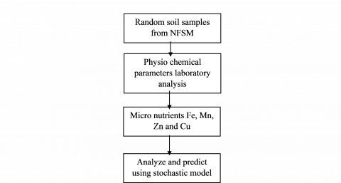
This research has proposed an efficient feature that affects the agriculture growth by different micro and macro nutrient level like Fe, Mn, Zn and Cu by adopting statistical model and techniques of data mining. In general, the novel SWD model is proposed for analyzing as well as predicting the factors affecting the agricultural growth and to increase the nutrients level which mean the expected agriculture increases using the strength of soil nutrients. Figure 1 has shown an overall block diagram of proposed stochastic model.
Figure 1. Overall block diagram of proposed model
A SWD model has initiated a process for evaluating probability adoptions of possible results by considering discretionary assortment in no less than one commitment over the time. The random variable is generally focused on fluctuations detected in historical data for a selective period by default time-series methods. This model is epistemic uncertainties over the variable has been considered whereas the uncertainties happen because of natural variation present in the process are modeled [21, 22]. Indeed, quantitative variable plays a major role by change in values present in the time series datasets. Moreover, the variable values present in the discrete random variable have accomplished by counting but in the case of continuous random variable accomplish by estimating [22]. Thus, the significant features available in the random variable are done by count.
However, the Weibull distribution of three-parameter may be accomplished from a Weibull distribution of two-parameter by leading the position or threshold parameter θ. Hence, there are three-parameter such as θ>0, β>0 and $\propto<\alpha<-\propto$ have GR distribution with CDF is expressed in Eq. (1).
$F(x ; \theta, \beta, \alpha)=\left[1-e^{-\left(\frac{(x-\theta)}{\beta}\right)^\alpha}\right] ; x>\theta, \beta, \alpha>0$ (1)
Here satisfy θ>0 and then β>0 be the form and range parameters, in that order. The equivalent probability density function (PDF) is expressed in Eq. (2).
$F(x ; \alpha, \lambda, \mu)=\alpha \beta^{-\alpha}(x-\theta)^{\alpha-1} e^{-\left(\frac{(x-\theta)}{\beta}\right)^\alpha}$ (2)
The respective survival function is formulated in Eq. (3).
$\bar{H}(X)=1-\left[1-e^{-\left(\frac{(x-\theta)}{\beta}\right)^\alpha}\right]=\left[1-e^{-\left(\frac{(x-\theta)}{\beta}\right)^\alpha}\right]$ (3)
Based on Weibull distribution of three parameters have considered with randomly in time is shown in Eq. (4). Considering the shape parameter as θ = 1.
$P\left(x_i<y\right)=\int_0^{\infty} g_k(x) \bar{H}(X) d x$
$=\int_0^{\infty} g_k(x)\left[e^{\left.-\left(\frac{(x-\theta)}{\beta}\right)^\alpha\right]} d x\right.$
$=\left[g^* \theta\left(\frac{1}{\beta}\right)^\alpha\right]$ (4)
The probability of survival function may provide an accumulative threshold has been failed only at subsequent time t.
s(t) = P(T > t) Probability of overall damage survived over time t.
$=\sum_{k=0}^{\infty} P\{\text {there are extractly } k \text { contacts }(0, t)\}^* P\{\text {the total cumulative threshold }(0, t)\}$
This can be obtained from renewal process represented in Eq. (5).
P (exact k policy decisions at (0, t)) = Fk(t) - Fk+1(t) with F0(t)=1.
$P(T>t)=\sum_{k=0}^{\infty} V_k(t) P\left(x_i<y\right)$
$=\sum_{k=0}^{\infty}\left[F_k(t)-F_{k+1}(t)\right]\left[g^*(\theta(1 / \beta))^\alpha\right]^k$ (5)
At present, the life time is defined by P(T<t) = L(t) = the life time distribution (T) is shown in Eq. (6).
$L(t)=1-S(t)$
$=1-\sum_{k=0}^{\infty}\left[F_k(t)-F_{k+1}(t)\right]\left[g^*(\theta(1 / \beta))^\alpha\right]^k$ (6)
Taking Laplace transformation L(t) is shown in Eq. (7).
$l^*(s)=\frac{1-\left[g^*(\theta(1 / \beta))^\alpha\right]\,\,^k f(s)}{1-g^*(\theta(1 / \beta))^\alpha f(s)}$ (7)
Let us consider the random variable indicating inter arrival that understand the exponential with parameter.
Now $f^*(s)=\frac{\lambda}{\lambda+s}$ is substituted in the Eq. (7) we get resulted is shown in Eq. (8).
$=\frac{1-\left[g^*(\theta(1 / \beta))^\alpha\right]\,^k\left(\frac{\lambda}{\lambda+s}\right)}{1-g^*(\theta(1 / \beta))^\alpha\left(\frac{\lambda}{\lambda+s}\right)}$
$l^*(s)=\frac{\lambda\left[1-\left[g^*(\theta(1 / \beta))^\alpha\right]\,^k\right]}{\left[\lambda+s-g^*(\theta(1 / \beta))^\alpha \lambda\right]}$ (8)
Consider the derivatives of first order in the Eq. (8), we get resulted is shown in Eq. (9).
$\left.\frac{d^* l(s)}{d s}\right|_{s=0}$
Given $s=0$
$\begin{gathered} E(A G)=\frac{1}{\lambda\left[1-g^*(\theta(1 / \beta))^\alpha\right]} \\ =\frac{1}{\lambda\left[1-g^*(\theta)^\alpha g^*(1 / \beta)^\alpha\right]} \\ g^*(\theta) \sim \exp (\theta), g^*(\theta)=\frac{\beta}{\beta+\theta} \\ g^*(1 / \beta)=\frac{\beta}{\beta+(1 / \theta)} \end{gathered}$ (9)
On simplification we get resulted is shown in Eq. (10).
$E(A G)=\frac{1}{\lambda\left[1-\left(\frac{\beta}{\beta+\theta}+\frac{\beta}{\beta+(1 / \theta)}\,\,\, \right)^\alpha\right]}$ (10)
The normalization by feature scaling is working with features in various data units and sizes as well as this movement is essential. Highlight scaling is a technique for formalizing the independent variables or data features scope [23, 24]. It's also known as data normalization in data handling but it has been usually done during the data preparation step to maintain all values in the range [0, 1] is illustrated in Eq. (11). This is also known as "unity-based standardization that can be summarized as limiting the values range in the dataset among all self-assertive point ‘a' and ‘b', as well as assigning (0.1, 0.9).
$X^{\prime}=a+\frac{\left(X-X_{\min }\right)(b-a)}{X_{\max }-X_{\min }}$ (11)
The projected stochastic Eq. (10) and normalization Eq. (11) have been utilized in the subsequent pseudo code. In this technique, the essential inputs are obtained from primary time series datasets in Table 1, which are then processed by the pseudo code below with the code subsequently delivering several expected parameters influencing agriculture growth estimation.
Table 1. Agricultural micro and macro nutrients soil content level from NFSM
|
Soil Sample |
Fe (%) |
Mn (%) |
Zn (%) |
Cu (%) |
|
S1 |
4.75 |
0.92 |
0.42 |
1.43 |
|
S2 |
3.17 |
1.42 |
1.22 |
0.91 |
|
S3 |
3.0 |
1.81 |
0.46 |
1.62 |
|
S4 |
1.17 |
0.62 |
0.86 |
0.3 |
|
S5 |
2.08 |
1.0 |
0.86 |
0.23 |
|
S6 |
1.08 |
1.19 |
0.26 |
0.23 |
|
S7 |
1.08 |
0.38 |
0.08 |
0.23 |
|
S8 |
2.83 |
1.46 |
0.2 |
0.42 |
|
S9 |
2.25 |
1.31 |
0.82 |
0.75 |
|
Limits |
>4% |
>4% |
>4% |
>4% |
Algorithm for normalization and SWD model
START
Initializing parameter of the model
Step:1 SET n $\leftarrow$ 9
Step:2 SET β $\leftarrow$ Fe [4.75, 3.17, 3.0, 1.17, 2.08, 1.08, 1.08, 2.83, 2.25]
Step:3 SET θ $\leftarrow$ Mn [0.92, 1.42, 1.81, 0.62, 1.0, 1.19, 0.38, 1.46, 1.31]
Step:4 SET α $\leftarrow$ Zn [0.42, 1.22, 0.46, 0.86, 0.86, 0.26, 0.08, 0.2, 0.82]
Step:5 SET λ $\leftarrow$ Cu [1.43, 0.91, 1.62, 0.3, 0.23, 0.23, 0.23, 0.42, 0.75]
INPUT: Parameters selected for SWD model is β, θ, α, λ
OUTPUT: Expected features which influence the growth of agriculture
Step:6 Generating control sequence by Eq. (12)
for i $\leftarrow$ 1 to n do
SET a $\leftarrow$ 0.1 and SET b¬ 0.5
for j $\leftarrow$ 1 to n do
beta[j]
$\leftarrow a+((\beta[j]-\operatorname{Min}(\beta))(b-a)) /(\operatorname{Max}(\beta)-\operatorname{Min}(\beta))$
RETURN beta
end for
for j$\leftarrow$ 1 to n do
delta[j]
$\leftarrow a+((\theta[j]-\operatorname{Min}(\theta))(b-a)) /(\operatorname{Max}(\theta)-\operatorname{Min}(\theta))$
RETURN delta
end for
for j$\leftarrow$ 1 to n do
theta[j]
$\leftarrow a+((\theta[j]-\operatorname{Min}(\theta))(b-a)) /(\operatorname{Max}(\theta)-\operatorname{Min}(\theta))$
RETURN theta
end for
for j$\leftarrow$ 1 to n do
alpha [j]
$\leftarrow a+((\alpha[j]-\operatorname{Min}(\alpha))(b-a)) /(\operatorname{Max}(\alpha)-\operatorname{Min}(\alpha))$
RETURN alpha
end for
for j$\leftarrow$ 1 to n do
lambda [j]
$\leftarrow a+((\lambda[j]-\operatorname{Min}(\lambda))(b-a)) /(\operatorname{Max}(\lambda)-\operatorname{Min}(\lambda))$
RETURN lambda
end for
Step:7 Generating preliminary sequences by Eq. (11)
SET count $\leftarrow$ 1
SET x $\leftarrow$ 1
while count < 9 do
PART1[x]$\leftarrow$ (beta[x]/ (theta[x]+ beta[x])) ^alpha[x])*lambda[x]
PART2[x]$\leftarrow$ ((beta[x]* theta[x])/ (1+beta[x]*theta[x])) ^alpha[x])*lambda[x]
EAG[x] $\leftarrow$ (1/ (lambda[x] - PART1+PART2))
RETURN EGA
x+1 and count+1
End while
End
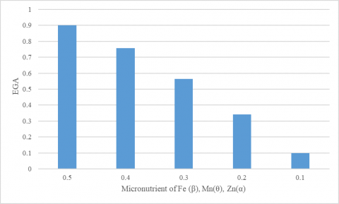
The physical parameters of such soil include soil moisture, soil pH, soil temperature was identified by physico-chemical properties. Basic soil chemical characteristics were determined in the analyzed soil samples such as EC, OC and OM. One of the soil parameters is micronutrient in which the elements are Fe, Cu, Zn, Mn. These parameters are collected from soil sample were present in seven various districts of Thiruvarur. The normalized dataset is appropriate to uniform range of data from 0.1 to 0.5 as well as assigning it in symbolic representation. The agriculture growth of primary field is based on micronutrient level such as the Fe is allocated as ‘β’. In addition, other field’s Mn is allocated as ‘θ’, Zn represented as ‘α’ and Cu is represented as ‘λ’. According to this hypothesis, it is very beneficial to apply numerical values definitely to the SWD model. The normalization and stochastic model equation also entirely solved using the above pseudo code techniques. Table 2 and Figure 2 show the normalized form of data using stochastic model occurs a decreasing EGA based on decreasing value of β, θ, α and fixed value of λ.
Table 2. Expected Prediction using β, θ, α (decrease) and λ (fixed)
|
Fe (%) β |
Mn (%) θ |
Zn (%) α |
Cu (%) λ |
EAG |
|
0.5 |
0.5 |
0.5 |
0.2 |
0.9000 |
|
0.4 |
0.4 |
0.4 |
0.2 |
0.7563 |
|
0.3 |
0.3 |
0.3 |
0.2 |
0.5642 |
|
0.2 |
0.2 |
0.2 |
0.2 |
0.3425 |
|
0.1 |
0.1 |
0.1 |
0.2 |
0.1000 |
Figure 3 and Table 3 have illustrated the normalized form of data using stochastic model occurs a decreasing EGA based on fixed value of λ, θ, α and decreasing of β.
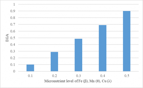
Table 4 and Figure 4 shows the normalized form of data using stochastic model occurs an increasing EGA based on fixed value of λ, θ, β and increasing of α.
Figure 2. Graphical representation of decreasing the Micronutrient level of Fe (β), Mn (θ), Zn (α) with decreasing EGA
Table 3. Expected prediction using θ, α, λ (fixed normal) and β (decrease)
|
Fe (%) β |
Mn (%) θ |
Zn (%) α |
Cu (%) λ |
EAG |
|
0.5 |
0.3 |
0.3 |
0.3 |
0.9000 |
|
0.4 |
0.3 |
0.3 |
0.3 |
0.6425 |
|
0.3 |
0.3 |
0.3 |
0.3 |
0.4166 |
|
0.2 |
0.3 |
0.3 |
0.3 |
0.2270 |
|
0.1 |
0.3 |
0.3 |
0.3 |
0.1000 |
Figure 3. Graphical representation of fixed Micronutrient level of Zn (α), Mn (θ), Cu (λ) with decreasing EGA
Table 4. Expected prediction using β, θ, λ (fixed normal) and α (increase)
|
Fe (%) β |
Mn (%) θ |
Zn (%) α |
Cu (%) λ |
EAG |
|
0.3 |
0.3 |
0.1 |
0.3 |
0.1000 |
|
0.3 |
0.3 |
0.2 |
0.3 |
0.2889 |
|
0.3 |
0.3 |
0.3 |
0.3 |
0.4867 |
|
0.3 |
0.3 |
0.4 |
0.3 |
0.6909 |
|
0.3 |
0.3 |
0.5 |
0.3 |
0.9000 |
Figure 4. Graphical representation of fixed micronutrient level of Fe (β), Mn (θ), Cu (λ) with increasing EGA
The value of β, θ, α are decreases (0.5 to 0.1) whereas the value of λ remain fixed normal (0.2). In this case EGA decreased. In order to increase the agriculture growth, the respective micronutrient level of Fe, Mn and Zn needs to improvise the characteristics by adding the chemical fertilizers like Ferrous sulphate, Manganese sulphate and Zinc sulphate based on the proportions are illustrated in Table 4. Similarly, the value of θ, α, λ as fixed normal, whereas the value of β is found decreasing (0.5 to 0.1). In this case EGA decreased. In order to increase the agriculture growth, the respective micronutrient of level of Fe needs to improvise the characteristics by adding the chemical fertilizers like Ferrous sulphate. The value of β, θ, λ fixed normal (0.2) whereas the value of α is found increasing (0.1 to 0.5). In this case EGA increased. Furthermore, when α and β values as decreases from range (0.5 to 0.1) and λ, θ values are increases (0.1 to 0.5) whereas the condition of EGA is decreased as well as increased by SWD model. In order to increase the agriculture growth, the respective micronutrient level of Fe, Mn and Zn needs to improvise the characteristics by adding the chemical fertilizers like Ferrous sulphate, Manganese sulphate and Zinc sulphate based on the proportions present in the nutrient range as shown in Table 5.
Table 5. Chemical fertilizers and nutrients range
|
Elements |
Fertilizers |
Content |
|
Iron |
Ferrous sulphate |
19% Fe |
|
Manganese |
Manganese sulphate |
30.5% Mn |
|
Boron |
Borax |
10.50% B |
|
Zinc |
Zinc sulphate |
21% Zn |
|
Copper |
Copper sulphate |
24% Cu |
The proposed stochastic model is the best choice for agriculture and evaluated to predict and validate agriculture growth using primary time series datasets. However, the growth of agriculture increases or decreases based on strength of micronutrient levels such as Fe, Mn, Cu and Zn. Hence the proposed stochastic model assists to identify the level of micronutrient present in the soil and also identify the agriculture growth by varying the micronutrient element present in the soil. Thus, this novel model recommended the fertilizers based on decrease in agriculture growth. The value of β, θ, α is decreases (0.5 to 0.1) whereas the value of λ remain fixed normal (0.2). In this case EGA decreased. In order to increase the agriculture growth, the respective micronutrient level of Fe, Mn and Zn needs to improvise the characteristics by adding the chemical fertilizers like Ferrous sulphate, Manganese sulphate and Zinc sulphate based on the proportions present in the nutrient range. The proposed pattern of stochastic is not only applicable in the fields of agricultural data analysis. The model accepts some other area like climate change and medical diagnosis. In future, the agriculture development can be predicted by the SWD method that is used to analyze the dataset include agriculture production, rainfall, groundwater and temperature.
[1] Rajesh, P., Karthikeyan, M. (2017). A comparative study of data mining algorithms for decision tree approaches using WEKA tool. Advances in Natural and Applied Sciences, 11(9): 230-243.
[2] Wikipedia. (2019). Economy of India. https://en.wikipedia.org/wiki/Economy of India#cite note-153, accessed on May 22, 2022.
[3] Nafidi, A., Bahij, M., Gutiérrez-Sánchez, R., Achchab, B. (2020). Two- parameter stochasticweibull diffusion model: Statistical Inference and application to real-modeling-example. Maths., 8(2): 160. https://doi.org/10.3390/math8020160
[4] Papajorgji, P.J., Pardaols, P.M. (2009). Data Mining in Agriculture. Springer Optimization and Its Applications.
[5] Rajesh, P., Karthikeyan, M. (2019). Data mining approaches to predict the factors that affect the agriculture growth using stochastic model. Int. J. Com. Sci. & Eng., 7: 18-23.
[6] Rajesh, P., Karthikeyan, M., Arulpavai, R. (2019). Data mining algorithm to predict the factors for agricultural development using stochastic model. International Journal of Recent Technology and Engineering, 8(3): 2713-271. https://doi.org/10.35940/ijrte.C4963.098319
[7] Rajesh, P., Karthikeyan, M. (2019). Data assimilation of gross domestic product (GDP) in India using stochastic data mining approach. Journal of Computational and Theoretical Nanoscience, 16(4): 1478-1484. http://dx.doi.org/10.1166/jctn.2019.8061
[8] Rajesh, P., Karthikeyan, M. (2019). Prediction of agriculture growth and level of concentration in paddy - a stochastic data mining approach. Advances in Intelligent Systems and Computing, Springer, 750: 127-139. https://doi.org/10.1007/978-981-13-1882-5_11
[9] Esary, J.D., Marshall, A.W. (1973). Shock models and wear processes. Ann. Probab., 1(4): 627-649. https://doi.org/10.1214/aop/1176996891
[10] Bravo-Ultra, B.E., Riegger, L. (1991). Dairy farm efficieency measurement using stochastic frontier and neo-classical duality. Am. J. Agric. Econ., 73: 421-428. https://doi.org/10.2307/1242726
[11] Uno, Y., Prasher, S.O., Lacroix, R., Goel, P.K., Karimi, Y., Viau, A., Patel, R.M. (2005). Artificial neural networks to predict corn yield from Compact Airborne Spectrographic Imager data. Computers and Electronics in Agriculture, 47(2): 149-161. https://doi.org/10.1016/j.compag.2004.11.014
[12] Bocca, F.F., Henrique, L., Rodrigues, A. (2016). The effect of tuning, feature engineering, and feature selection in data mining applied to rainfed sugarcane yield modelling. Comput. Electron. Agric., 128: 67-76. https://doi.org/10.1016/j.compag.2016.08.015
[13] Rathod, S., Singh, K.N., Patil, S.G., Naik, R.H., Ray, M., Meena, V.S. (2018). Modeling and forecasting of oilseed production of India through artificial intelligence techniques. Indian J. Agric. Sci., 88(1): 22-27.
[14] Omran, S.A. (2016). A stochastic simulation model to early predict susceptible areas to water table level fluctuations in North Sinai, Egypt. The Egyptian Journal of Remote Sensing and Space Science, 19(2): 235-257. 2016. https://doi.org/10.1016/j.ejrs.2016.03.001
[15] Murugesan, R., Sudarsanam, S.K., Ganesan, M., Vijayakumar, V., Neelanarayanan, V., Venugopal, R., Rekha, D., Saha, S., Bajaj, R., Miral, A., Malolan, V. (2019). Artificial intelligence and agriculture 5.0. International Journal of Recent Technology and Engineering, 8(2).
[16] Patil, P., Panpati, V., Kokate, S. (2020). Crop prediction system using machine learning algorithms. International Research Journal of Engineering and Technology (IRJET), 7(2): 748-753.
[17] Osco, L.P., Ramos, A.P.M., Pinheiro, M.M.F., et al. (2020). A machine learning framework to predict nutrient content in valencia-orange leaf hyperspectral measurements. Remote Sensing, 12(6): 906. https://doi.org/10.3390/rs12060906
[18] Anand, S., Silviya Catherine, J., Shanmuga Priya, S., Sweatha, A. (2019). Monitoring of soil nutrients using IoT for optimizing the use of fertilizers. International Journal of Science, Engineering and Technology Research, 8(4).
[19] Manjula, E., Djodiltachoumy, S. (2017). Data mining technique to analyze soil nutrients based on hybrid classification. IJARCS, 8(8). https://doi.org/10.26483/ijarcs.v8i8.4794
[20] Rajak, R.K., Pawar, A., Pendke, M., Shinde, P., Rathod, S., Devare, A. (2017). Crop recommendation system to maximize crop yield using machine learning. International Research Journal of Engineering and Technology, 4(12): 950-953.
[21] Boser, B.E., Guyon, I.M., Vapnik, V.N. (1992). A training algorithm for optimal margin classifiers. In Proceedings of the Fifth Annual Workshop on Computational Learning Theory, pp. 144-152. https://doi.org/10.1145/130385.130401
[22] Dalla Mura, M., Benediktsson, J.A., Waske, B., Bruzzone, L. (2010). Morphological attribute profiles for the analysis of very high resolution images. IEEE Trans. Geosci. Remote. Sens., 48(10): 3747-3762. https://doi.org/10.1109/TGRS.2010.2048116
[23] Renda, A., Barsacchi, M., Bechini, A., Marcelloni, F. (2019). Comparing ensemble strategies for deep learning: an application to facial expression recognition. Expert Syst. Appl., 136: 1-11. https://doi.org/10.1016/j.eswa.2019.06.025
[24] Tan, K., Wang, H., Zhang, Q., Jia, X. (2018). An improved estimation model for soil heavy metal (loid) concentration retrieval in mining areas using reflectance spectroscopy. J. Soils Sediments, 18(5): 2008-2022. https://doi.org/10.1007/s11368-018-1930-6