Giulia Cervelli* | Luca Parrinello | Claudio Moscoloni | Giuseppe Giorgi
© 2022 IIETA. This article is published by IIETA and is licensed under the CC BY 4.0 license (http://creativecommons.org/licenses/by/4.0/).
OPEN ACCESS
Appropriate design of marine structures, such as offshore facilities and harbours, requires a detailed estimation of synthetic wave parameters. Inaccuracies and unreliability of wave data have implications in many aspects of marine engineering, such as structural strength, cost, and design. In this paper, a critical analysis of the most common data acquisition methods is made, focusing on in-situ instrumentation and numerical models. Considering the Pantelleria island as case study, records of a proprietary wave buoy and the ERA5 dataset of ECMWF (European Centre for Medium-Range Weather Forecasts) have been compared. This paper first highlights the methods and challenges of offshore experimental campaigns for wave monitoring and eventually presents a critical and quantitative comparison of the two approaches (experimental versus numerical), highlighting their respective advantages and disadvantages.
buoy, ECMWF portal, ERA5 dataset, in-situ measurements, sea states analysis, wave
The main hydraulic phenomena occurring in the coastal region are waves. Specifically, friction between the wind and the sea surface is the leading cause of wave generation [1]. Since waves induced by wind are generally characterized by a maximin period of 30 seconds, they are called short waves. This clarification allows differentiating the waves caused by the wind and by the tides. In fact, the periodicity of waves caused by tides have a hourly order of magnitude, and they are defined as long waves.
In the field of marine engineering, both short than long waves are fundamental for a multitude of applications [2, 3]: in the port design, for example, information on short waves is used to determine the loads acting on the structure, while long waves are used to calculate the excursion of the sea surface concerning the mean level [4]. Knowing the loads acting on the structures is crucial to verify the stability of port the under operating conditions and check that the maximin damage is limited under extreme conditions. As far as tides are concerned, they play a fundamental role in water pull: during low tide, the vertical distance between the free surface and the seabed is reduced compared to high tide. In order to correctly design a port, it is necessary to avoid ships getting stuck in the seabed and therefore, it is necessary to know exactly the characteristics of long waves.
In maritime engineering, the need to predict sea conditions is linked with many needs: first and foremost, the waves continually break on the coasts, and these impact public safety and trade, recreational activities and, of course on navigation. The research towards wave prediction has pushed for more than two decades to devise increasingly reliable models to navigate safely and to have adequate inputs for the design coastal structures. The study of the sea is the basis of the activities related to the design of offshore structures [5, 6], the study of sediment transport [7] as well as analyzing coastal flooding [8] and obviously identifying regions with exploitable energy [9]. Moreover, offshore wind, floating solar, waves, tides, and currents have a high energetic potential of interest [10] and wave information is requested for design and analysis. Indeed, exploiting renewable energy in the sea would support the energy transition and accelerate the decarbonization process.
To develop offshore technologies, the sea's information, particularly the waves and wind, is essential and several methodologies can provide such metocean data [11]. For example, broad interest is devoted to measurements of salinity [12] or current profiles [13], since they are essential for identifying the movements of oceanic water masses, and the use of reliable instrumentation is critical. In addition, for efficient underwater communication, appropriate systems are necessary when instruments are placed on the seabed and data are required as time passes. Among the various methods, OFDM (Orthogonal Frequency-Division Multiplexing) and MIMO (Multiple Input Multiple Output) technologies are a good solution, providing high data transfer rates [14]. At the same time, using an antenna suitable for communications is necessary, and taking advantage of an ultrawideband instrument is often a good solution [15]. To date, a multitude of disadvantages characterizes each source of metocean data. In economic and temporal terms, high costs are some of the problems related to in situ survey campaigns.
This paper supports maritime stakeholders for choosing the metocean data source: in-situ instruments, satellite observations and numerical models are described in detailed. By understanding the limits of applicability, advantages and disadvantages of different data sources, the most suitable choice of data source can be made: depending on the objective, different temporal and spatial resolutions, accuracy, and reliability levels are needed. Offshore facilities can be considered the perfect example of how crucial wave data are and how the data characteristics needed vary depending on the stage of project development [16]. The project's first phase involves site selection [17], and several locations must be compared to identify the optimal one. For reasons of time and cost, numerical model data, which are easy to obtain and inexpensive, are usually used. On the other hand, the actual design phase requires using accurate data representative of the study site, and in-situ instrumentation is preferable to other sources. On the other hand, maintenance and decommissioning require forecast of sea states, and numerical models are the best choice [18]. Through state-of-the-art considerations and comparisons between measured and modelled data, in addition to the strengths and weaknesses of the different sources, are emphasized.
The paper is structured as follows: Section 2 introduces the synthetic parameters describing the waves; in Section 3, the different data sources are introduced and compared; in Section 4, the case study is presented, describing the island of Pantelleria, the installed instrumentation, and data provided by ECMWF. Then, in Section 5, the methodology is described, and in Section 6, the analysis is presented. Finally, Section 7 draw some final conclusions and remarks.
Short waves can be described using several synthetic parameters [11, 19]: the most representative are the significant wave height Hs, the energy period Te, the mean direction Dirm and the directional width s. These parameters allow to describe each individual sea state fully. In particular, sea waves are largely studied via the two-dimensional wave spectrum S(ω,θ) [19], i.e. the distribution of energy over frequencies and directions. This parameter provides a complete statistical description of the waves and, from a theoretical point of view, can be obtained as the product of the spectrum of frequencies S(ω) [20] and directions D(θ) [21, 22]:
$S(\omega ,\theta )=S(\omega )D(\theta )$ (1)
As with any statistical distribution, the shape of a wave spectrum is usually expressed in terms of moments: the n-th order moment mn, of the variance density S(ω) is defined by:
${{m}_{n}}=\int\limits_{0}^{\infty }{{{f}^{n}}S(\omega )d\omega }$ (2)
Starting from the general momentum mn definition, and considering, in general, the spectrum, the synthetic parameters of interest can be obtained as:
${{H}_{s}}=4\sqrt{{{m}_{0}}}$ (3)
${{T}_{e}}=\frac{{{m}_{-1}}}{{{m}_{0}}}$ (4)
$Di{{r}_{m}}=\arctan \frac{\int\limits_{0}^{2\pi }{\int\limits_{{{\omega }_{\min }}}^{{{\omega }_{\max }}}{\sin \theta S(\omega ,\theta )d\omega d\theta }}}{\int\limits_{0}^{2\pi }{\int\limits_{{{\omega }_{\min }}}^{{{\omega }_{\max }}}{\cos \theta S(\omega ,\theta )d\omega d\theta }}}$ (5)
$s=\frac{2}{\int_{-\pi}^{\pi}\left[2 \sin \left(\frac{1}{2}\left(\operatorname{Dir}-\operatorname{Dir}_{m}(\omega)\right)\right)\right]\quad^{2} D(\theta) d \theta}-1$ (6)
Eq. (3), (4) and (5) are widely used; Eq. (6), on the other hand, is less known and has been obtained starting from the relationship that links directional spreading with directional width and considering the definition of directional spreading [11].
Several data sources are available to obtain the synthetic parameters of interest: in-situ records, satellite measurements, and numerical modelling.
Theoretically, an ideal data source provides data with high information content, reliable, accurate and representative of the site of interest. Unfortunately, the above requirements are never satisfied simultaneously, and each different data source realizes a different trade-off. High information content refers to the amount of information obtained from the source. The optimal parameter is the frequency and directional spectrum S(ω,θ). Alternatively, synthetic parameters are acceptable. Among the different data acquisition methods, only the use of data measured by satellites is disadvantageous in terms of information content. Data obtained from satellite records are provided as products with different levels of processing [23]:
Up to Level 2 the data can be considered instrumental; thereafter, they are obtained from numerical modelling. In addition to mathematical formulations, another difference concerns the information content: the only available parameter concerning Level 2 is the significant wave height. All other synthetic parameters describing the waves are provided by the following Levels, which fall into modelled data.
Regarding the reliability requirement, only satellite and modelled data have this characteristic. The wave information recorded by in-situ instrumentation has the disadvantage of operating intermittently: due to a multitude of recurring problems caused by malfunctions, failures, sapped batteries and downtime due to maintenance. These gaps are unpredictable and unavoidable, and thus the time series obtained from in-situ instrumentation are often characterized by missing data.
3.1 In-situ measurement
The in-situ instrumentation records the temporal evolution of sea states and they can be placed above the sea surface or submerged. The main instruments are:
Once the data has been recorded, users can acquire them through different transmission techniques (e.g. via radio, GSM, satellite) or in person. The submerged devices cannot use any data connection, and it is necessary to recover the instrument and manually download the acquired data periodically.
The most reliable sources are wave buoys [24, 25], i.e. floating devices with anchoring elements placed on the seabed. They provide wave information; however, modern buoys also measure wind speed [26]. This type of instrumentation can be classified concerning the method of operation:
Generally, one of the major limits of the buoy is linked to the depth: they can only be installed in shallow water, around 40 m deep, since they must be moored.
As for the operational life, it is closely related to the number of battery packs installed, the amount of data transmitted, and the frequency of transmission. For simple battery pack equipment, the operating life is of the order of a few months (typically from 6 to 18).
3.2 Satellite observation
Earth Observation satellites are an already available solution to study ocean behavior in specific regions of interest. Dedicated earth observation satellites provide dataset concerning ocean condition, according different level of processing. Among the main instrumentation installed on the satellites, the Radio Altimeter (RA) [27] and Synthetic Aperture Radar (SAR) [28] are the most widely used for extrapolating wave parameters from space.
Once the on-board instruments have performed the measurements, the subsequent extrapolation of the parameters depends mainly on the processing method applied to these measurements.
Since the data stream generated is very high, usually the instrument does not continuously send data to receiving stations on Earth, but it does so intermittently. To date, satellite information is not yet fully exploited: they are just used for the calibration and validation of wave numerical models.
3.3 Numerical model
The numerical modelling allows to simulate coastal hydrodynamics and they can be differentiated into two macro-categories: physical models and mathematical models. Physical models consist of a physics reproduction of the study system, generally on a reduced scale, while the latter is represented by a system of equations that describe the behaviour of the phenomena under analysis. Furthermore, the mathematical models can be distinguished into physically-based models or conceptual models. The former is based on the detailed description of the physics of phenomena and often is represented by differential equations. The latter places the parameters of interest in a simplified relationship, leading to less complex modelling.
The present study highlights the differences concerning in-situ measured data and the opensource data available from the ECMWF portal. In particular, the considerations based upon the data comparison can be used to define how and when a category of source is better than another. To achieve this objective, the Pantelleria island has been chosen as the case study. The data obtained from the buoy installed near the North-West coast are compared with the ERA5 dataset [29].
4.1 Pantelleria island
The site of analysis is located near the North-West coast of the island of Pantelleria. It has a volcanic nature and emerged about 324,000 years ago [30]; the island consists of the emerged summit of an imposing submarine volcanic building and its maximum height is 836 m.
Pantelleria is located almost in the center of the Sicilian Channel, together with the Pelagie islands; this area is characterized by a trend of irregular bathymetric and variable depths. The Sicilian channel, in fact, has two deep thresholds, respectively 500 m towards the Tyrrhenian Sea and 600 m towards the Ionian Sea. Only in the central area are higher depths reached due to some depressions, such as the Pantelleria Basin, with a maximum depth of 1317 m. Pits therefore separate the island from the continental shelf.
Figure 1 shows the buoy installation site, on the North-West coast of the island of Pantelleria.
Figure 1. Pantelleria area
4.2 Datawell Waverider DWR-G
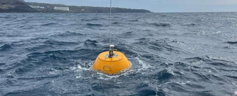
The buoy used for recording wave information is a Datawell Waverider DWR-G: this instrument is equipped with a Global Positioning System (GPS) module that allows the measurement of directional waves. The buoy (Figure 2), whose hull is characterized by a spherical shape, can measure frequencies up to 0.01 Hz (corresponding to a wave period of 100 s), while the size of the buoy itself limits its high frequency response. Indeed, if the wavelength is less than the size of the buoy, the buoy is unable to follow the wave profile and the observed data is not representative of the wave condition.
Figure 2. Datawell Waverider DWR-G
Furthermore, the low frequency force to which the system is subjected is determined by the hydrodynamic properties of the buoy itself in combination with its mooring.
Specifications are shown in Table 1, extracted from the Datawell Waverider DWR-G manual.
Table 1. Specifications of Datawell Waverider DWR-G
|
Heave, north, west |
Value |
|
Range |
-20 m – +20 m |
|
Resolution |
1 cm |
|
Accuracy |
± 1 cm or 0.1% of value, whichever is worse |
|
Period time (frequency range) |
1.6 s – 100 s (0.01 Hz – 0.64 Hz) |
|
Direction |
Value |
|
Range |
0° – 360° |
|
Resolution |
1.5° |
|
Accuracy |
1.5° |
|
Reference |
True north (WGS84) |
|
Filter |
Value |
|
Sampling frequency |
2.0 Hz |
|
Digital filtering type |
Phase-linear, combined band-pass and single-integrating FIR filter |
|
Filter delay |
256.0 s |
|
Decimation filter delay |
43.0 s |
|
HF output buffer delay and actual HF output |
5.5 s (approximately, does not apply to logger files) |
|
Data output rate |
1.28 Hz |
|
Band-pass characteristics |
0.0154 – 0.59 Hz: 0.0013dB 0.0132 Hz: 0.009dB 0.0115 Hz: 0.09dB 0.01 Hz: 0.8dB low frequency side: 52dB/octave(<0.01Hz) |
To measure the direction of the wave, the buoy is based on a disc shape positioned at the pivot point of its movement, which follows the two-dimensional shape of the wave. By monitoring the pitch and roll angles of the buoy and its lifting motion, it is possible to characterize the incident wave fully.
The Datawell Waverider DWR-G is equipped with a sensor package that measures the accelerations along the x, y, z axes, the magnetic field along these axes and the pitch and roll movements.
4.2.1 Buoy data processing
The buoy measures raw North, West and vertical displacements at a constant rate of 1.28 Hz. Such displacements are to be intended as excursions concerning the average position of the buoy, and are used to obtain processed data for the description of the sea state. In particular, the vertical displacement of the buoy is used to obtain a power spectral density (PSD) of the wave amplitude, showing what wave amplitudes occur at what frequencies. If also North and West displacements are included in the analysis, it is possible to obtain waves directional spectrum, by conducting the calculation of the Fourier series of the three signals, and then the PSD, as in the previous case.
The data format in which the data are acquired form the buoy is called the real-time format. It consists of long-existing hexadecimal vectors containing information about vertical, North and West displacements and also words forming the spectrum and system files. The real-time format is organized at four levels:
1. Vectors of 64 bits, containing real-time data together with cyclical data;
2. Blocks of 18 vectors assembling cyclical data with spectral and system data;
3. Spectrum file, constituted by the spectral data of 16 blocks;
4. System file, constituted by the system data of 16 blocks;
Each 64-bit vector is divided into three parts: the first contains cyclical data (regarding the system file or the spectrum file), the second contains the real-time displacement in vertical, North and West directions, and the third part contains information on transmission errors and corrections.
With respect to the timing of the data, each vector of 64 bits covers one acquisition (at the frequency of 1.28 Hz, or 0.78125 s); each block contains 18 vectors, equivalent to 14.0625 s of data acquisition; each file contains 16 blocks (or 288 vectors) with 225 s of data; finally, each full cycle contains 8 repeated files, or equivalently 30 minutes of data acquisition. It is worth to underline that in a full cycle are contained 30 minutes of displacement data for the buoy, while the spectrum data are invariant during the 30 min time span. Specifically, during half an hour, 8 spectra of 200 s data interval each are collected and averaged. At the end of the half hour, over which the calculations are executed, all spectral parameters are available. The spectrum is transmitted 8 times during the next half-hour for redundancy.
4.3 ECMWF
Numerical models, such as atmospheric and oceanic models from ECMWF (European Centre for Medium-Range Weather Forecasting), provide many environmental datasets. It was founded in 1975 with the aim of producing global medium-term weather forecasts by pooling various scientific and technological resources. The center therefore started from the goal of developing numerical models capable of making predictions and allowing free access to such data.
The ERA5 database [29] of ECMWF is among the most used databases in marine analysis and provides several time series: wave, wind, solar and much other information can be obtained. However, the spatial resolution corresponding is not suitable for accurate calculations: the ERA5 database provides wave parameters with a spatial resolution of 0.5°x0.5° (about 50 km x 50 km). In addition, the complicated orography of the Mediterranean Sea further reduces the accuracy of the wind parameters. Consequently, since waves are generated by the interaction between the wind and the sea surface, and since numerical models exploit this correlation, the ERA5 wave data are less accurate in the Mediterranean basin than in other locations.
Generally, ERA5 data are often used as input to calculate more accurate data by applying additional numerical models specific to coastal regions.
Synthetic wave parameters provided by ERA5 were used to compare measured data from the buoy with modeled data.
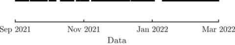
Data recorded by the DWR-G buoy were acquired and post-processed to obtain the synthetic parameters of interest. These parameters are the significant wave height Hs, the energy period Te, the mean direction Dirm, and the directional width s. The buoy was installed in early September 2021 with 12 months of expected life; however, failures of the battery packs led to an early decommissioning by early March 2022. Moreover, the communication between the transmitting and receiving antenna were subject to seldom interruption. Overall, this led to a partial much loss of data.
Figure 3 represents the time series of the available data obtained from the buoy. Compared to the total number of registrations that would have occurred between the beginning of September 2021 and the end of February 2022, the data loss is around 17%.
Figure 3. Buoy time series
The time series provided by the ECMWF were acquired concerning the same time period as the buoy recordings, with the minimum available time resolution i.e. every hour. To assess the datasets similarities and differences, the time series were overlaid and occurrences bivariate diagrams were produced. In addition, parameter comparison using scatters was made in both synchronous and asynchronous modes.
The synthetic parameters of the buoy were compared with those acquired from the ECMWF portal. The first difference that distinguishes them concerns the temporal resolution of the data: the information of the wave recordings is provided every half an hour, while the modelled data has an hourly resolution. Because of this difference, several analyzes were carried out. The comparison of the historical series was carried out by comparing all the available data. Similarly, the wave roses and the occurrences bivariate diagrams were calculated and compared considering the whole set of recorded and modelled data. Subsequently, the capabilities of the ECMWF model to reproduce sea states were investigated in greater detail: the data sets used were manipulated and the data corresponding to the gaps present in the recordings was discarded from the time series obtained from numerical modelling. As for the recorded data, they have been selected to have a single parameter every hour. Then, a homogeneous comparison of the hourly sea states was performed from the beginning of September 2021 to the end of February 2022.
6.1 Complete time series
Time series overlays of the significant wave height Hs (Figure 4), the energy period Te (Figure 5), and the directional width s (Figure 6), concerning the two datasets under consideration, have been obtained. Visualization of the time series is helpful to appreciate the variability of the parameters as time passes. Significant wave height Hs obtained from numerical modelling manage to describe the wave climate with good detail. In fact, from the superposition shown in Figure 4 a similar trend is evident. However, the ERA5 data generally underestimate the recorded wave conditions.
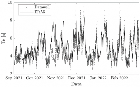
Similarly, the temporal evolution of the energy period Te is well represented by the ERA5 dataset, although usually, the values are lower (Figure 5). The only obvious exception is between mid-October and mid-November 2021, where the values obtained from the model overestimate the recorded data.
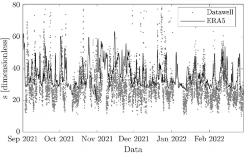
On the other hand, the directional width parameter s is not well calculated by the numerical model. The data obtained from the buoy have much higher variability than other data (Figure 6). This difference depends on the spatial resolution used by the numerical model. The directional width s describes the variability of the wave energy distribution in different directions; however, considering an extensive cell (0.5° x 0.5°) does not allow to obtain good information in terms of direction.
Figure 4. Time series of significant wave height Hs
Figure 5. Time series of energy period Te
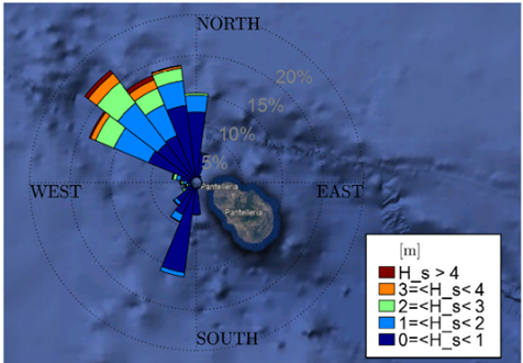
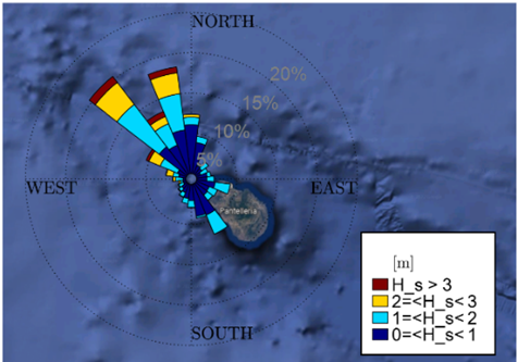
Figures 7 and 8 represent the wave rose, obtained from the buoy and ERA5 data, respectively. As expected, the roses are different: the polar plot obtained from the modelled data also predicts incoming waves from the South-East direction. This error depends on the spatial resolution of ERA5 data and on the island location: Pantelleria is located in the Sicilian Channel and this area is characterized by a wind that blows both from the Nort-West to South-East and viceversa. Since the wind generates the waves, also these have the corresponding directions. However, the site where the buoy has been installed is protected from the arrival of the southern waves: once they reach the island, they must circumnavigate it, changing direction. Depending on the application and the objectives, the direction of the waves can be a crucial parameter, and such significant errors may not be acceptable.
Figure 6. Time series of directional width s
Figure 7. Rose plot using buoy data
Figure 8. Rose plot using ERA5 data
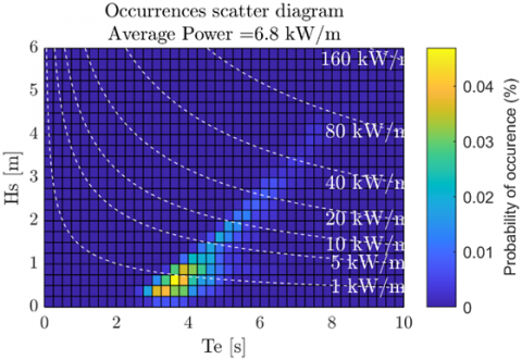
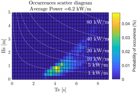
Occurrence scatters were identified to determine which sea states are most commonly occurring. Figure 9 represents the frequency of Hs-Te pairs recorded by the buoy: the most frequently occurring sea states have a wave height Hs of about 0.5 m and an energy period Te of nearly 4 s. The scatter obtained with the ERA5 data (Figure 10) shows similar characteristics despite a greater spread around the most occurring Hs-Te pair is evident.
Since the significant wave height and energy period obtained from numerical modeling generally underestimate the real values, the wave power is also lower. Considering the values of the recorded data, the average wave power is 6.8 kW/m, while in the case of the ERA data it is 6.2 kW/m.
Figure 9. Occurrences scatter using buoy data
Figure 10. Occurrences scatter using ERA5 data
6.2 Matching time series
In order to compare the measured data with modelled ones, through scatter plots, homogenization of the data was necessary. Subsequently, both synchronous and asynchronous analyses were conducted to evaluate the simultaneity of the recorded sea states with the calculated ones.
6.2.1 Synchronous analysis
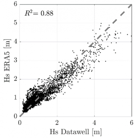
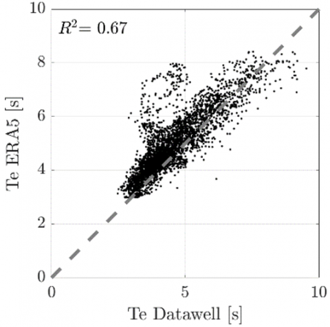
Synchronous analysis are conducted by comparing the homogenized hourly time series. The same number of data characterizes these new time series: each hourly sea state recorded by the buoy has been compared with that calculated by numerical modelling. Figures 11, 12 and 13 represent the scatters of the significant wave height Hs, the energy period Te, and the directional spreading s, respectively. The bisector is represented in all scatters to facilitate the graphs' interpretation. The conformity of the data is described numerically by the value of the R2: high values, tending towards unity, indicate a good adherence between the data, low values, tending to zero, on the other hand, refer to poor conformity.
The significant wave height is well calculated by the model, in particular, for low values of Hs, the model tends to overestimate slightly, while for higher values, the model tends to underestimate the real ones. The conformity of the data is confirmed by the value of the R2, which is approximately 0.9.
Concerning the energy period, the value of the R2 is lower than that obtained for the significant wave height and it is equal to 0.67, indicating a more significant deviation between the recorded and modelled data. Figure 12, in fact, shows a cloud of points above the bisector due to the overestimation of the parameter during the period October-November 2021.
Figure 11. Significant wave height time series
Figure 12. Significant wave height time series
Figure 13 shows the correlation between the measured and modelled directional width values: a high dispersion around the bisector is evident, and the R2 value confirms the poor fit of the data. As expected, in fact, the modelled data do not correctly describe reality.
Figure 13. Significant wave height time series
6.2.2 Asynchronous analysis
Asynchronous analyses were conducted to verify that the differences from the synchronous analyses did not depend on homogenization. In particular, the new data sets were obtained considering the maximum values of Hs, Te and s, recorded in time windows of 12 h. The new data was released from the reference time, and any time lags were ignored.
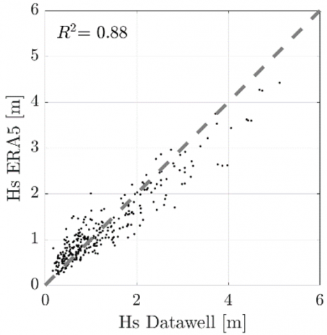
Figures 14, 15 and 16 show the scatter plot of the significant wave height Hs, the energy period Te and the directional width s, respectively.
Figure 14. Significant wave height time series
Figure 15. Significant wave height time series
Figure 16. Significant wave height time series
Both the points distribution and the values of R2 are similar to what is determined by the synchronous analysis and this shows that there is no time lag of the sea states. In particular, the conformity of data from the model and in-situ instrumentation is confirmed by the R2value of about 0.9. As in the synchronous analysis, the model overestimates the lower wave heights and underestimates the higher ones. Regarding the energy period, a scattering of the cloud around the bisector is evident, and the model tends to overestimate the periods near 4s, referring to the October-November 2021 period. Figure 16 shows the correlation of directional width values, obtained by asynchronous analysis, between the measurements and the model. The scatter around the bisector shows a poor correlation, confirmed by the R2 value of 0.09.
This document aims to support maritime stakeholders in identifying the most suitable wave data source. The synthetic parameters necessary to describe the characteristics of the sea states are introduced. Subsequently, state-of-the-art concerning the different existing methodologies for acquiring the synthetic parameters is described.
In addition to the presentation of the methodology, a case study was investigated: the sea states recorded and modeled concerning the island of Pantelleria were evaluated. The measured dataset was obtained from the Datawell Waverider DWR-G buoy, installed near the island's North-West coast. The available time series describes the period from the beginning of September 2021 to the end of February 2022. Except for some losses, the time series is quite robust. The data obtained from numerical modeling and available on the ECMWF portal were acquired for comparison. In particular, the dataset of the significant wave height Hs, of the energy period Te, the mean direction Dirm and of the directional width s of ERA5, with hourly resolution, was obtained.
The comparison between the time series was carried out in the analyses. Among the most evident results, it emerged that the ERA5 generally underestimates both the significant wave height and the energy period. The main reason is linked to the complex orography of the Mediterranean Sea and the consequent difficulty in modelling the winds. The wave datasets of ERA5, in fact, are obtained based on an environmental model of wind reproduction, which underestimates the wind speed in closed basins.
The directional width obtained from numerical modelling, on the other hand, loses veracity for extreme values, both lower and higher: this is mainly since directionality analyzes are highly dependent on the location of analysis. Since the spatial resolution of the ERA5 data is 0.5° x 0.5° (approximately 50 km x 50 km), the ability to describe geographic features is absent. In fact, near the coasts, the interaction between the seabed is incisive and shoaling and reflection phenomena modify the direction of the wavefront and all the other characteristics.
The difficulty of the wave model used by ECMWF to obtain correct directions is also confirmed by comparing the wave roses. In the case of the graph depicting the modelled data, a multitude of waves have a direction coming from the mainland. Obviously, this result is not physically possible and confirms a loss of reliability.
Regarding the scatters, they confirmed what emerged from the other analyzes. Furthermore, comparing the scatters of the synchronous analyzes with those of the asynchronous ones, it emerged that ERA5 could provide the wave parameters without any time lag, then, wave propagation occurs without delaying or anticipating the arrival of sea states.
The errors generated by using ECMWF data have practical implications: harbour design and wave energy exploitation are just a few examples where underestimation of significant height peaks and incorrect wave period and directional width could lead to design errors and malfunctions. Since synthetic wave parameters have many uses, depending on the objectives, it is possible to determine from which source to acquire them. Indeed, in the emergence of renewable energy from waves, a detailed assessment of sea states is fundamental to designing and optimizing wave energy converter [31-33] of offshore wind turbines [34]. This activity generally involves installing recording equipment at sea, and economic efforts must be made. Furthermore, the experimental campaigns require a waiting time of at least one year in order to obtain a suitable time series for making assessments on sea states; at the same time, the recorded data are often used to calibrate and validate numerical models, and therefore, to obtain more extended time series. However, to install devices at sea, it is necessary to follow bureaucratic procedures that slow down the activities.
Given the complexity associated with obtaining measured data, the conscious and sensible choice of the installation site is fundamental. To identify the most energetic sea site, it is necessary to process a large amount of data. To this end, the data obtainable from ECMWF are suitable for analysis. Therefore, the time series are hourly and can adequately describe the evolution of sea states. All synthetic parameters and many others are available free of charge for approximately 40 years. Furthermore, as emerged from the analyses, the modelled data described both the significant wave height and the energy period. The average direction and the directional width, on the other hand, must be carefully evaluated and the information must be considered indicative.
[1] Lighthill, M.J. (1962). Physical interpretation of the mathematical theory of wave generation by wind. Journal of Fluid Mechanics, 14(3): 385-398. https://doi.org/10.1017/S0022112062001305
[2] Sigmund, S., El Moctar, O. (2018). Numerical and experimental investigation of added resistance of different ship types in short and long waves. Ocean Engineering, 147: 51-67. https://doi.org/10.1016/j.oceaneng.2017.10.010
[3] Guerrini, M., Bellotti, G., Fan, Y., Franco, L. (2014). Numerical modelling of long waves amplification at Marina di Carrara Harbour. Applied Ocean Research, 48: 322-330. https://doi.org/10.1016/j.apor.2014.10.002
[4] Antonini, A., Archetti, R., Lamberti, A. (2017). Wave simulation for the design of an innovative quay wall: the case of Vlorë Harbour. Natural Hazards and Earth System Sciences, 17(1): 127-142. https://doi.org/10.5194/nhess-17-127-2017
[5] Cervelli, G., Carapellese, F., Bracco, G., Mattiazzo, G. (2021). Variability of wecs’ performance according to the wave directional spreading variation. In Proceedings of the 14th European Wave and Tidal Energy Conference, pp. 2288-1. EWTEC. ISSN 2706-6940.
[6] Sirigu, S. A., Foglietta, L., Giorgi, G., Bonfanti, M., Cervelli, G., Bracco, G., Mattiazzo, G. (2020). Techno-Economic optimisation for a wave energy converter via genetic algorithm. Journal of Marine Science and Engineering, 8(7): 482. https://doi.org/10.3390/jmse8070482
[7] Gonzalez Santamaria, R., Zou, Q.P., Pan, S.P. (2011). The impact of a wave farm on large scale sediment transport. Conference: European Wave and Tidal Energy Conference.
[8] Wolf, J. (2009). Coastal flooding: Impacts of coupled wave–surge–tide models. Natural Hazards, 49(2): 241-260. https://doi.org/10.1007/s11069-008-9316-5
[9] Rusu, E., Soares, C.G. (2009). Numerical modelling to estimate the spatial distribution of the wave energy in the Portuguese nearshore. Renewable Energy, 34(6): 1501-1516. https://doi.org/10.1016/j.renene.2008.10.027
[10] Appiott, J., Dhanju, A., Cicin-Sain, B. (2014). Encouraging renewable energy in the offshore environment. Ocean & Coastal Management, 90: 58-64. https://doi.org/10.1016/j.ocecoaman.2013.11.001
[11] Holthuijsen, L.H. (2010). Waves in Oceanic and Coastal Waters. Cambridge University Press.
[12] Le Menn, M., Malardé, D., David, A., Brault, P., Grosso, P., de Bougrenet de la Tocnaye, J.L., Le Reste, S., Podeur, C. (2016). Development of an optical salinometer for oceanography. Instrumentation Mesure Métrologie, 15(1-2): 53-63. https://doi.org/10.3166/I2M.15.1-2.53-63
[13] Komen, G. (1992). Operational analysis and prediction of ocean wind waves. By M.L KHANDEKAR. Springer, 1989. 214 pp. DM 77. Guide to Wave Analysis and Forecasting. World Meterological Organization, 1988. 206 pp. SFR 47. Journal of Fluid Mechanics, 234: 692-693. https://doi.org/10.1017/S0022112092220978
[14] Le Menn, M., Morvan, S. (2020). Perfecting of a calibration bed for current profilers. Instrumentation Mesure Métrologie, 19(3): 179-184. https://doi.org/10.18280/i2m.190302
[15] Pallavi, C.H., Sreenivasulu, G. (2021). A high speed underwater wireless communication through a novel hybrid opto-acoustic modem using MIMO-OFDM. Instrumentation Mesure Métrologie, 20(5): 279-287. https://doi.org/10.18280/i2m.200505
[16] Medina-Lopez, E., McMillan, D., Lazic, J., et al. (2021). Satellite data for the offshore renewable energy sector: synergies and innovation opportunities. Remote Sensing of Environment, 264: 112588. https://doi.org/10.1016/j.rse.2021.112588
[17] Sempreviva, A.M., Barthelmie, R.J., Pryor, S.C. (2008). Review of methodologies for offshore wind resource assessment in European seas. Surveys in Geophysics, 29(6): 471-497. https://doi.org/10.1007/s10712-008-9050-2
[18] Dowell, J., Zitrou, A., Walls, L., Bedford, T., & Infield, D. (2013, September). Analysis of wind and wave data to assess maintenance access to offshore wind farms. In European Safety and Reliability Association Conference, pp. 743-750. https://doi.org/10.1201/b15938-114
[19] World Meteorological Organization (WMO). (1998). Guide to Wave Analysis and Forecasting. WMO, 2020 (2018 edition).
[20] Alves, J.H.G., Banner, M.L., Young, I.R. (2003). Revisiting the Pierson–Moskowitz asymptotic limits for fully developed wind waves. Journal of Physical Oceanography, 33(7): 1301-1323. https://doi.org/10.1175/1520-0485(2003)033<1301:RTPALF>2.0.CO;2
[21] Goda, Y. (1999). A comparative review on the functional forms of directional wave spectrum. Coastal Engineering Journal, 41(1): 1-20. https://doi.org/10.1142/S0578563499000024
[22] Krogstad, H.E., Barstow, S.F. (1999). Directional distributions in ocean wave spectra. In the Ninth International Offshore and Polar Engineering Conference. OnePetro.
[23] Drusch, M., Del Bello, U., Carlier, S., et al. (2012). Sentinel-2: ESA's optical high-resolution mission for GMES operational services. Remote sensing of Environment, 120: 25-36. https://doi.org/10.1016/j.rse.2011.11.026
[24] Liu, Q., Lewis, T., Zhang, Y., Sheng, W. (2015). Performance assessment of wave measurements of wave buoys. International Journal of Marine Energy, 12: 63-76. https://doi.org/10.1016/j.ijome.2015.08.003
[25] Niclasen, B.A., Simonsen, K. (2007). Note on wave parameters from moored wave buoys. Applied Ocean Research, 29(4): 231-238. https://doi.org/10.1016/j.apor.2008.01.003
[26] Kelberlau, F., Neshaug, V., Lønseth, L., Bracchi, T., Mann, J. (2020). Taking the motion out of floating lidar: Turbulence intensity estimates with a continuous-wave wind lidar. Remote Sensing, 12(5): 898. https://doi.org/10.3390/rs12050898
[27] Vignudelli, S., Birol, F., Benveniste, J., Fu, L.L., Picot, N., Raynal, M., Roinard, H. (2019). Satellite altimetry measurements of sea level in the coastal zone. Surveys in Geophysics, 40(6): 1319-1349. https://doi.org/10.1007/s10712-019-09569-1
[28] Heimbach, P., Hasselmann, K. (2000). Development and application of satellite retrievals of ocean wave spectra. Elsevier Oceanography Series, 63: 5-33. https://doi.org/10.1016/S0422-9894(00)80003-3
[29] Hersbach, H., Bell, B., Berrisford, P., et al. (2020). The ERA5 global reanalysis. Quarterly Journal of the Royal Meteorological Society, 146(730): 1999-2049. https://doi.org/10.1002/qj.3803
[30] Agnesi, V., Federico, C. (1995). Aspetti geografico-fisici e geologici di Pantelleria e delle Isole Pelagie (Canale di Sicilia). Naturalista siciliano, 19: 1-22.
[31] Drew, B., Plummer, A.R., Sahinkaya, M.N. (2009). A review of wave energy converter technology. Proceedings of the Institution of Mechanical Engineers, Part A: Journal of Power and Energy, 223(8): 887-902. https://doi.org/10.1243/09576509JPE782
[32] Giorgi, G., Sirigu, S.A., Bonfanti, M., Bracco, G., Mattiazzo, G. (2021). Fast nonlinear Froude–Krylov force calculation for prismatic floating platforms: a wave energy conversion application case. Journal of Ocean Engineering and Marine Eenrgy, 7: 439-457. https://doi.org/10.1007/s40722-021-00212-z
[33] Bonfanti, M., Hillis, A., Sirigu, S.A., Dafnakis, P., Bracco, G., Mattiazzo, G., Plummer, A. (2020). Real-time wave excitation forces estimation: An application on the ISWEC device. Journal of Marine Science and Engineering, 8(10): 825. https://doi.org/10.3390/jmse8100825
[34] Fenu, B., Attanasio, V., Casalone, P., Novo, R., Cervelli, G., Bonfanti, M., Sirigu, S.A., Bracco, G., Mattiazzo, G (2020). Analysis of a gyroscopic-stabilized floating offshore hybrid wind-wave platform. Journal of Marine Science and Engineering, 8(6): 439. https://doi.org/10.3390/jmse8060439