Ahmed Sami Naser | Wisam Abdulabbas Abidalla*
© 2022 IIETA. This article is published by IIETA and is licensed under the CC BY 4.0 license (http://creativecommons.org/licenses/by/4.0/).
OPEN ACCESS
In this research, the time series were analysed for four gauges (Mosul, Baghdad, Kut, and Husayabah) using autoregressive (AR) models with constant and periodic autoregressive coefficients. It was found that the best model for Mosul, Baghdad, and Husaybah gauges is AR (2) with periodic autoregressive coefficients, while the best model for the Kut gauge was AR (2) with constant autoregressive coefficients. The test was also suggested to determine the most appropriate model based on the values of autocorrelation of residuals (independent normal variable) and it was compared with the drawings of correlograms of autocorrelation of residuals rk(ξ) and with two tests: the AIC test and the portmanteau lack test. It was concluded that the suggested test was more accurate and more reliable.
water discharge, surface water, time series, forecasting, confidence limit
In hydrology, the time series analysis becomes a major tool. It is using for building mathematical models to generate synthetic hydrologic records to forecast the hydrologic events and to fill in missing data with extend records [1]. The hydrologic processes such as runoff and rainfall evolve on a continues time scale in which recording gauging station in a river provides a continuous record of water discharge through time. Time series forecasting comes when making scientific predictions based on the historical time of data, which involves building models through a historical analysis and using them for making observations and driving future strategic decision-making [2].
In forecasting, an important distinction is that at the time of the work, the future outcome is completely unavailable and can be estimated through a careful analysis with evidence-based priors [3]. Application of statistical hydrology in the past few days was restricted to problems of surface water, especially in the case of analysing hydrologic extremes such as floods, droughts, etc. In addition, during the past three decades, in hydrology, the statistical domain has broadened with the advent of computing technology to encompass the problems in each surface water and groundwater system. Statistics have been found to be a powerful tool for analysing hydrologic time series [4]. The main aim of time series analysis is to describe and detect quantitatively each of the generating processes underlying the given sequence of observations. In hydrology, the analysis of time series is used to construct mathematical models to generate records of synthetic hydrologic events, to forecast hydrologic events, to find trends and shifts in hydrologic records, and to fill in missing data and extend records [5].
The main aim of time series analysis is to describe and detect quantitatively each of the generating processes underlying the given sequence of observations. In hydrology, the analysis of time series is used to construct mathematical models to generate records of synthetic hydrologic events, to forecast hydrologic events, to find trends and shifts in hydrologic records, and to fill in missing data and extend records [6].
The measurement of surface water flow is a very important aspect in hydrology-related projects such as forecasting, the monitoring of water quality and flood studies, geomorphology, and aquatic life support, amongst others [7]. It is the most common requirement for management and planning of any project in water resources [8]. Availability of long-term streamflow data covering many years is required for the appropriate hydrological studies [9]. Most hydrological data, such as rainfall and water discharge, are subject to a certain degree of randomness. Since simulation and improvement of any water resource system requires specifying data in order to complete the process of designing or simulating a particular hydraulic facility, this requires the generation of future data, and this generated data depends on the analysis of historical time series, which led to the emergence of many models in order to generate forecast time series [10]. These models were required in order to generate expenditures for the purpose of designing a particular dam, planning to manage dam reservoirs, designing a specific bridge and other hydraulic installations [11], or developing a strategic plan for the purpose of managing the water resources of a particular country in the future. Hence the importance of generating data in the planning and operation of water resource systems or the design of a hydraulic plant.
The other aspect, which is included in the importance of generation, is finding reliability as well as determining the amount of risk for any hydraulic facility in dams. For example, as a future strategic plan, determining the number of expenses and comparing them to the needs of a specific country requires determining the degree of risk in the future. One of the well-known and used models is AR1, AR2, which will be the subject of this study in the country of Iraq.
Therefore, the study employs AR (1) and AR (2) with the two cases of constant coefficient and periodic coefficient to analyse data for stations (Mosul, Baghdad, and Kut located on the Tigris River and Husaybah located on the Euphrates River) in order to generate data for future years and determine the appropriate model for each measuring station by using. The main objective of this study is also to propose a new statistical test model that elicits the number of correlation functions for residual points that fall outside the confidence limit.
2.1 Study area
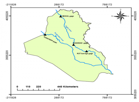
The study area (area of data collection) is located at the water discharge measuring stations located on the Tigris River in the cities of Mosul, Baghdad, and Kut, as well as located on the Euphrates River in the city of Husayabah in western Iraq, as shown on the map in Table 1 and Figure 1.
Table 1. Location of discharge measuring stations
|
Stream Gage |
Location |
|
Mosul |
Latitude 36° 37′ 57″ N, Longitude 42° 49′ 03″ E. |
|
Baghdad |
33° 24′ 34″ N, Longitude 44° 20′ 32″ E |
|
Kut Barrage |
Latitude 32° 29′ 00″ N, Longitude 45° 50′ 00″ E |
|
Husabah |
Latitude 34° 25′ 20″ N, Longitude 41° 00′ 38″ E |
Figure 1. Area of case study (Discharge measuring stations)
2.2 Time series modeling
Homogeny time series transform to normal distribution (Yt) is required for stability the variance and improving the normality assumption of the noise series [12].
$Y v, \tau=g \tau(X v, \tau)$ (1)
where: gτ is the transformation function used to transform it to normal, and then the inverse transformation of Yt will used to get the generated non-normal series Xt.
$X v, \tau=g-1(Y v, \tau)$ (2)
where: g-1(Yv,τ) is the invers transformation function. There are many methods to transformed data to normal, one of these is the original form of Box-Cox transformation [13].
$g(\lambda)=\left\{\begin{array}{cc}\frac{\chi^{\lambda}-1}{\lambda} \\ \ln \chi\end{array} \quad \begin{array}{r}\text { if } \lambda \neq 0 \\ \text { if } \lambda=0\end{array}\right.$ (3)
in which, value of λ assume from ( -1 to +1, step 0.1) to find optimum λ, it should find the relationship between skewness (cs) and λ with assumption relationship is polynomial second order as shown below:
$\lambda=a_{0}+a_{1} c_{s}+a_{2} c s^{2}$ (4)
So, the optimum λ where cs = 0, then λ = a0. To find (a0, a1, a2), it was using polynomial regression between λi and csi by solving these matrices:
$\left[\begin{array}{ccc}n_{\lambda} & \sum C_{S} & \sum C_{S}{ }^{2} \\ \sum C_{S} & \sum C_{S}^{2} & \sum C_{S}{ }^{3} \\ \sum C_{S}{ }^{2} & \sum C_{S}{ }^{3} & \sum C_{S}^{4}\end{array}\right]\left[\begin{array}{l}a_{0} \\ a_{1} \\ a_{2}\end{array}\right]=\left[\begin{array}{c}\sum \lambda_{i} \\ \sum C_{S i} \lambda_{i} \\ \sum C_{S i} \lambda_{i} 2\end{array}\right]$ (5)
2.3 AR models
Autoregressive (AR) models, one of the most important methods in which used for forecasting especially in hydrology and water resources so as to discharge forecasting. It will review the periodic AR models that are modeled with constant coefficients or modeled with periodic coefficients. The periodic normal series (Y v,τ) can be written as [12]:
$Y v, \tau=\mu \tau+\sigma \tau Z v, \tau$ (6)
where: Y v,τ = gτ (Xv,τ), µτ and στ are the periodic mean and periodic standard deviation, and (Z v,τ) is the time dependent series with mean zero and variance one.
2.3.1 AR models with constant autoregressive coefficient
The time dependent (Zv,τ) represented by AR models with constant autoregressive coefficient. For AR (1) model [12]:
$Z_{t}=\Phi_{1} Z_{t-1}+\varepsilon_{t}$ (7)
For AR (2) model:
$Z_{t}=\Phi_{1} Z_{t-1}+\Phi_{2} Z_{t-2}+\varepsilon_{t}$ (8)
In general, the AR(P) model:
$Z_{t}=\Phi_{1} Z_{t-1}+\cdots \quad \Phi_{P} Z_{t-P}+\varepsilon_{t}$ (9)
where:
t = (v -1) w + τ
v = no. of years; τ= 1,2, 3…., w; w = number of time interval in years (w = 12 month); ΦP = the i th partial autocorrelation coefficients; εt = the residual or error (assumed normal with mean zero and variance σ2ε) or (the normal independent variable (white noise) with standard deviation σε). Since (εt = σε 2. ξ) in which ξ is an independent normal variable with zero mean and variance one [12].
For AR (1):
$\sigma_{\varepsilon}^{2}=\frac{N \cdot \sigma^{2}}{(N-1)}\left\{1-\emptyset_{1}^{2}\right\}$ (10)
$\mathop{\varphi }_{1}={{r}_{1}}\quad $ (11)
For AR (2):
$\mathop{\sigma }_{\varepsilon }^{2}=\frac{N.\mathop{\sigma }^{2}.\left( 1+\mathop{\varphi }_{2} \right)}{\left( N-2 \right)\left( 1-\mathop{\varphi }_{2} \right)}\left\{ {{\left( 1-\mathop{\varphi }_{2} \right)}^{2}}-\mathop{\varphi }_{1}^{2} \right\}$ (12)
$\mathop{\varphi }_{1}=\frac{\mathop{r}_{1}.\left( 1-\mathop{r}_{2} \right)}{\left( 1-\mathop{r}_{1}^{2} \right)}\quad ;\quad \mathop{\varphi }_{2}=\frac{\mathop{r}_{2}^{{}}-\mathop{r}_{1}^{2}}{\left( 1-\mathop{r}_{1}^{2} \right)}$ (13)
$\mathop{\sigma }_{\mathop{{}}^{{}}}^{2}=\frac{1}{\left( N-1 \right)}\sum\limits_{t=1}^{N}{{{\left( {{Y}_{t}}-\bar{Y} \right)}^{2}}\mathop{{}}^{{}}}$ (14)
2.3.2 AR models with periodic autoregressive coefficient
The time dependent (Zv,τ) represented by AR models with periodic autoregressive coefficients [12].
For AR (1) model:
$Z_{v, \tau}=\Phi_{1, \tau} Z_{v, \tau-1}+\sigma_{\varepsilon, \tau} \xi_{v, \tau}$ (15)
For AR (2) model:
$Z_{V, \tau}=\Phi_{1, \tau} Z_{V, \tau-1}+\Phi_{2, \tau} Z_{v, \tau-2}+\sigma_{\varepsilon, \tau} \xi_{v, \tau}$ (16)
In general, the AR(P) model as the form:
$Z_{v, \tau}=\Phi_{1, \tau} Z_{v, \tau-1}+\cdots \Phi_{P, \tau} Z_{v, \tau-P}+\sigma_{\varepsilon, \tau} \xi_{v, \tau}$ (17)
where, the $\left(\Phi_{j}, \tau^{\prime} \mathrm{s}\right)$ are the periodic autoregressive coefficient and $\sigma_{\varepsilon}$ periodic variance of the residuals.
For AR (1):
Φ1, τ= ρ 1, τ; τ = 1, 2…,12; ρ1, τ = periodic correlation coefficients.
For AR (2):
$\mathop{\varphi }_{1,\tau }=\frac{\mathop{\rho }_{1,\tau }-\mathop{\rho }_{1,\tau -1}\quad.\quad\mathop{\rho }_{2,\tau }}{1-\mathop{\rho }_{1}^{2}}$ (18)
$\mathop{\varphi }_{2,\tau }=\frac{\mathop{\rho }_{2,\tau }-\mathop{\rho }_{1,\tau }.\mathop{\rho }_{1,\tau -1}}{1-\mathop{\rho }_{1,\tau -1}^{2}}$ (19)
where, τ = 1, 2…,12
The periodic variance of the residual for AR (1) and AR (2) can be written as in equations (20) and (21) respectively [12]:
$\mathop{\sigma }_{\varepsilon \tau }^{2}=1-\mathop{\varphi }_{1,\tau }.\mathop{\rho }_{1,\tau }$ (20)
$\mathop{\sigma }_{\varepsilon \tau }^{2}=1-\mathop{\varphi }_{1,\tau }.\mathop{\rho }_{1,\tau }-\mathop{\varphi }_{2}.\mathop{\rho }_{2,\tau }$ (21)
3.1 Data collection
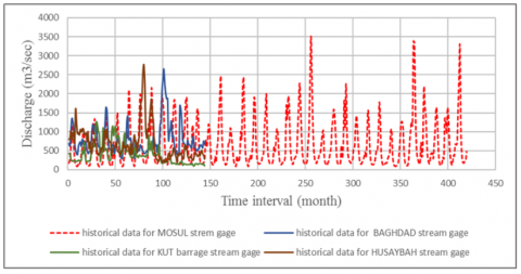
Series of water discharge data were collected for Tigris River at stream gage stations in the cities of Mosul, Baghdad, and Kut, and for Euphrates River at stream gage stations in the city of Husaybah [11]. These data were presented in the form of graphs, as shown in Figure 2. The data in Figure 2 included the monthly water discharge recorded for the Tigris River at the (Mosul station which available for 35 years, Baghdad station for 12 years, Kut station for 12 years and for the Euphrates River at Husaybah station for 12 years).
Figure 2. The original historical data for (Tigris - Euphrates) rivers at Four Stream Gage Stations
3.2 Data generation
In this study, the generation of data by using AR (1) and AR (2) models with both constant-coefficient and periodic coefficients. The procedure to solve these models can be written by the following steps:
$t=\frac{{{{\bar{x}}}_{1}}-{{{\bar{x}}}_{2}}}{s.\sqrt{\frac{1}{{{n}_{1}}}+\frac{1}{{{n}_{2}}}}}$ (22)
$s={{\sqrt{\frac{\sum\limits_{i=1}^{{{n}_{1}}}{{{\left( {{x}_{i}}-{{{\bar{x}}}_{1}} \right)}^{2}}+\sum\limits_{j=2}^{{{n}_{2}}}{{{\left( {{x}_{j}}-{{{\bar{x}}}_{2}} \right)}^{2}}}}}{{{n}_{1}}+{{n}_{2}}-2}}}^{{}}}$ (23)
where:
$\bar{x}_{1}, \bar{x}_{2}:$ mean sample 1 and 2 respectively; n1, n2: number of data for sample 1 and sample 2; xi, xj: values of data for sample 1 and sample 2; t: is t – calculated. The t – calculated is compare with t – table with α = 0.97 S and degree of freedom = N-2 to decide the significant of existence the trend, and if it exist should be remove.
$\mathop{\mu }_{\tau }=\mu +\sum\limits_{j=1}^{h}{\left[ \mathop{\beta }_{j}\cos \left( \frac{2\pi i\tau }{w} \right)+\mathop{\alpha }_{j}\left( \frac{2\pi i\tau }{w} \right) \right]}$ (24)
where: τ= 1, 2…, w; αj, βj = Fourier series coeff.; j = the harmonic; h = total number of harmonic which is equal w / 2.
$\mathop{\beta }_{j}=\frac{2}{w}\sum\limits_{\tau =1}^{w}{\left[ \mathop{\mu }_{\tau }\cos \left( \frac{2\pi i\tau }{w} \right) \right]}$, j = 1……, h (25)
$\mathop{\alpha }_{j}=\frac{2}{w}\sum\limits_{\tau =1}^{w}{\left[ \mathop{\mu }_{\tau }\sin \left( \frac{2\pi i\tau }{w} \right) \right]}$, j = 1……, h (26)
where: w = h
${{\beta }_{h}}=\frac{1}{w}\sum\limits_{\tau =1}^{w}{\left[ \mathop{\mu }_{\tau }\cos \left( \frac{2\pi h\tau }{w} \right) \right]}$ (27)
And αh = 0; computing µτ and στ with only those harmonics which are significant according to variance analysis and F- test doing. When sure existing the periodicity, it should be removed it [12].
${{\varepsilon }_{\nu ,\tau }}=\frac{\mathop{yy}_{\nu ,\tau }-\mathop{\mu }_{\tau }}{\mathop{\sigma }_{\tau }}$ (28)
yyv,τ: data after transforming to normal; εv,τ: data after removing the periodicity. Then, ensure that the mean = 0 and σ = 1, if not it should be standardized.
onfidencelimits $=\frac{-1 \mp 1.96 \sqrt{N-K-1}}{\sqrt{N-K}}$ (29)
3.3 Statistical methods for choosing suitable model
There are many methods which give an impression to decide to choose fit a model or suitable model.
3.3.1 Akaike information criterion
The Akaike information criterion (AIC) is defined as [14]:
$\operatorname{AIC}(p, q)=N \cdot \ln (\sigma \varepsilon 2)+2(p+q)$ (30)
where: σε2 = variance of the residual series with N number of data.
For AR (1), P = 1; q = 0; So, AIC (1,0) = N.ln(σε2) + 2
For AR (2), P = 2; q = 0; So, AIC (2,0) = N.ln(σε2) + 4
The minimum value of AIC gives a better model.
3.3.2 Port Manteau lack of fit test
Test depending upon values of the autocorrelation coefficients of the residual rk(ξ) at lag k. The Q – Statistic defined as [15].
$Q=N \cdot \sum_{K=1}^{M} r_{K}^{2}(\zeta)$ (31)
where: rk(ξ) is the autocorrelation coefficients of the residual (ξ) at lag k; (M) is max. lag consider (N / 4). The model is accepted if the Q- calculated less than χ2 table with degree of freedom = m – p, and confidence limit = 95%.
3.3.3 New test
There are many conditions where the New Suggestion Test is dependent upon choosing the better model, which depends on the value of the autocorrelation coefficient of the residual rk(ξ) of lag k. Regarding the value of rk (ξ) it may be negative, positive, or zero value and be bound by upper and lower limits. Firstly, assuming the limits (upper or lower) are closed to rk (ξ) value, which is done according to the following conditions: If rk $\leq$ is zero, the absolute of rk(ξ) is subtracted from the absolute of the lower limit; if rk $>$ is greater than zero, the absolute of rk(ξ) is subtracted from the absolute of the upper limit.
In fact, in a process where the distance between rk (ξ) values and the limits is found, the products of these differences will be either negative or positive values. Negative values indicate that values are within the limits, but if values were positive, that indicates that values are outside the limits. To make this conclusion more practical, any negative values should be converted into mathematical equations whose result is zero (which means that the value is within limits). Regarding positive values, they should be converted into mathematical equations whose result is one (which means that the value is outside limits).
It was done by dividing these values (-or +) by the absolute value of the same value and adding (1). Finally, if you take the square root of the values, the result will be either zero or one. When summation for these was done, the result gave a number of rk (ξ) that was outside the limits. hoods, which give an impression of deciding to choose a model or suitable model.
$\begin{cases}\text { if } \operatorname{sing} & r_{k}(\zeta)<=0 \quad n^{\prime} \text { out } 1=\sum_{1}^{N / 4} \frac{1}{2}\left(\frac{C_{k}}{\left|C_{k}\right|}+1\right) \\ \text { if } \quad \operatorname{sign} & r_{k}(\zeta)>0 \quad n^{\prime} \text { out } 2=\sum_{1}^{N / 4} \frac{1}{2}\left(\frac{D_{k}}{\left|D_{k}\right|}+1\right)\end{cases}$ (32)
$N^{\prime}$ out $=n^{\prime}$ out $1+n^{\prime}$ out 2 (33)
where:
$C_{k}=\left|r_{k}(\zeta)\right|-\left|\frac{-1-1.96 \sqrt{N-k-1}}{\sqrt{N-k}}\right|$ (34)
$D_{k}=\left|r_{k}(\zeta)\right|-\left|\frac{-1+1.96 \sqrt{N-k-1}}{\sqrt{N-k}}\right|$ (35)
where, k=1,2,3, ... N/4.
$A C \%=\left(1-\frac{N \prime \text { out }}{\frac{N}{4}}\right) * 100$ (36)
For more accurate calculation, the accepted AC% is equal or greater than 95%. The decision for the better model was made when the number of rk (ξ) values outside the limits was the least. However, the percentage of the number of rk (ξ) must be greater or equal to 95% to indicate the better model. It also depends on the experience of the analyst.
4.1 Results of data generation
To generate the monthly flow discharge, a computer programme was written, using the available data for the gauges (Mosul, Baghdad, Kut, and Husaybah). The purpose is to generate a sample of 50 years using the AR (1) and AR (2) models and with two cases of a constant autoregressive coefficient and a periodic autoregressive coefficient for each model, and for the four gages. The programme is written in the form of a subroutine. The first subroutine includes a test of the homogeneity of the data. It includes checking the trend existing by using t-test Eq. (23) and t-table with a significant level of 0.975 and degree of freedom equal to (n-2) for the four gauges is 1.96, and comparing it with the t-calculated. It was found no trend exists for the four gauges because the t-calculated is less than the t-table, so there is no need to remove the trend and the data is homogeneous for all gages.
The second subroutine consisted of the test of normality of data. It was found the skewness (cs) for all gauges was greater than zero as shown in Table 2. Therefore, there was a need to transform the data using Eq. (3) to evaluate the optimum (λ) after finding the coefficients of the second-order polynomial equation for all gauges through Eq. (4) and Eq. (5). The optimum (λ) for the gauges is illustrated in the Table 2.
Table 2. Skewness and optimum (λ) for all gauges
|
Gauge |
Mosul |
Baghdad |
Kut |
Husaybah |
|
Skewness |
1.64 |
2.13 |
1.33 |
2.09 |
|
Optimum (λ) |
-0.142 |
-0.691 |
-0.263 |
-0.241 |
The third subroutine of the program, the periodicity, was analysed for six harmonics to determine µτ and στ using Eq. (24) to Eq. (27), using the variance analysis and F-test to indicate whether the periodicity exists or not. If the periodicity exists, we will find it µτ and στ, after specifying the harmonic number that is significant through explaining percent, we will remove the periodicity Eq. (28).
The test mean and standard deviation of the results should be zero and one, respectively, or they will be standardized. The result is (ε), which is the residuals after removing the periodicity and standardizing. From variance analysis, it was found that the periodicity existed for all gauges except Baghdad gauge, which didn’t have periodicity, and according to explain percent, it was found that the number of harmonics significant was 1,2,5, and 4. For example, the harmonics significant were 1,2,4, and 3. In Table 3 are also shown Fourier coefficients of fitted harmonics to means and standard deviations.
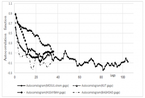
Finding the autocorrelation for the residual (ε). This was done in the fourth subroutine of the program, from lag equal one to lag (n/4). Figure 3 illustrates the relationship between lags and rk (ε).
Figure 3. Relationship between rk (ε) l and lags
From Eq. (11) and Eq. (13) it was determined the partial autocorrelation function for AR (1) and AR (2) models as constant. The results are shown in Table 4 for all gauges.
The fifth subroutine of the program, including the calculation of the periodic autocorrelation function with lag 1 and lag 2 for all gages, is illustrated in Table 5, which leads to the computation of the partial autocorrelation function for AR (1) and AR (2) models as periodic Ф. The results are shown in Table 6.
Table 3. Test periodicity, no. of harmonics, and Fourier coefficients for means and standard deviations
|
Gauges |
Test exist the periodicity |
Mean |
Standard deviation |
||||
|
Harmonic |
αi |
βi |
Harmonic |
αi |
βi |
||
|
Mosul |
exist |
1 |
0.448 |
-0.15 |
1 |
0 |
0.038 |
|
2 |
-0.082 |
0.065 |
2 |
0.004 |
0.018 |
||
|
3 |
0.016 |
0.007 |
3 |
-0.003 |
-0.006 |
||
|
4 |
-0.004 |
-0.008 |
4 |
0.003 |
-0.002 |
||
|
Baghdad |
Not exist |
_ |
_ |
_ |
_ |
_ |
_ |
|
Kut |
exist |
1 |
0.026 |
0.016 |
1 |
0.014 |
0.008 |
|
2 |
-0.007 |
0.01 |
2 |
0.002 |
0.013 |
||
|
5 |
0.003 |
-0.003 |
5 |
0.003 |
0.001 |
||
|
4 |
-0.002 |
-0.003 |
4 |
0.003 |
-0.002 |
||
|
Husayabh |
exist |
1 |
0.024 |
-0.014 |
1 |
-0.006 |
-0.02 |
|
2 |
-0.007 |
-0.017 |
2 |
0.004 |
0.001 |
||
|
4 |
-0.004 |
0.009 |
4 |
0 |
0.003 |
||
|
3 |
0.006 |
-0.001 |
3 |
-0.003 |
0.007 |
||
Table 4. Constant Ф1 for AR (1), constant Ф1 and Ф2 for AR (2)
|
Gauges |
Model |
Partial autocorrelation function |
||
|
Constant Ф |
Mosul |
AR (1) |
Ф1 |
0.614 |
|
AR (2) |
Ф1 |
0.531 |
||
|
Ф2 |
0.134 |
|||
|
Baghdad |
AR (1) |
Ф1 |
0.722 |
|
|
AR (2) |
Ф1 |
0.778 |
||
|
Ф2 |
-0.0785 |
|||
|
Kut |
AR (1) |
Ф1 |
0.894 |
|
|
AR (2) |
Ф1 |
0.904 |
||
|
Ф2 |
-0.0121 |
|||
|
Husaybah |
AR (1) |
Ф1 |
0.882 |
|
|
AR (2) |
Ф1 |
0.744 |
||
|
Ф2 |
0.156 |
|||
In Tables 7 and Table 8 it was calculated the variance (σε 2) of dependent stochastic component using AR (1) and AR (2) as constant Ф by Eq. (10) and Eq. (12), regarding periodic Ф the calculation of (σε 2) was used Eq. (20) and Eq. (21), this is done in sixth subroutine of the program.
In subroutine seventh through a tenth of the program and from Eq. (9). It was computed (ε) for AR (1) and AR (2) models with constant Ф, and periodic Ф has used Eq. (17).
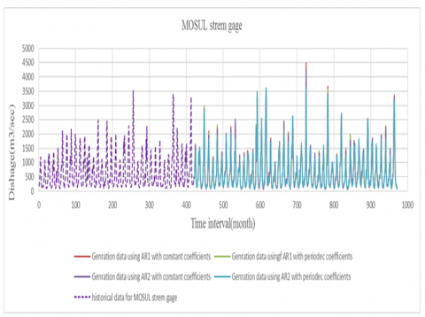
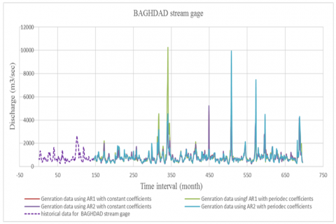
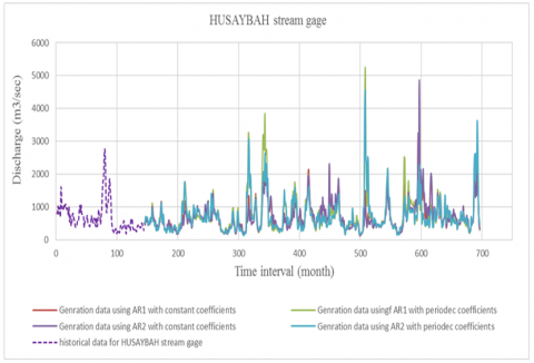
Using 600 standard normal random number for generating 50 years with eliminating 5 years data to avoid an error that produce due to an assumption of initial (z). It is done by Eq. (9) and Eq. (17) with substituting (εt = σε2. ξ) and (εt τ = σε τ 2. ξv,τ) respectively. Figure 4 to Figure 7 represented the data generated for all gages and for AR (1) and AR (2) models with constant Ф and periodic Ф. Discharges were generated for Mosul gage up to the year 2042, for Baghdad gage up to the year 2036, for Kut gage up to the year 2047, and Husaybah gauge up to the year 2038.
Figure 4. Data generation for Mosul gauge
Figure 5. Data generation for Baghdad gauge
Table 5. Periodic autocorrelation function
|
Gages |
Periodic autocorrelation function (lag 1 and lag2) |
Month |
|||||||||||
|
1 |
2 |
3 |
4 |
5 |
6 |
7 |
8 |
9 |
10 |
11 |
12 |
||
|
Mosul |
r1 |
0.379 |
0.538 |
0.542 |
0.552 |
0.761 |
0.878 |
0.968 |
0.949 |
0.956 |
0.227 |
0.347 |
0.536 |
|
r2 |
0.335 |
0.503 |
0.330 |
0.587 |
0.520 |
0.747 |
0.875 |
0.885 |
0.893 |
0.131 |
0.145 |
0.218 |
|
|
Baghdad |
r1 |
0.488 |
0.662 |
0.836 |
0.779 |
0.974 |
0.868 |
0.792 |
0.948 |
0.979 |
0.124 |
0.635 |
0.847 |
|
r2 |
0.481 |
0.364 |
0.669 |
0.457 |
0.757 |
0.819 |
0.531 |
0.648 |
0.892 |
0.046 |
0.176 |
0.663 |
|
|
Kut |
r1 |
0.942 |
0.967 |
0.895 |
0.978 |
0.952 |
0.928 |
0.953 |
0.991 |
0.991 |
0.488 |
0.964 |
0.907 |
|
r2 |
0.902 |
0.878 |
0.845 |
0.907 |
0.970 |
0.880 |
0.850 |
0.921 |
0.994 |
0.430 |
0.639 |
0.859 |
|
|
Husaybah |
r1 |
0.344 |
0.932 |
0.794 |
0.940 |
0.939 |
0.909 |
0.882 |
0.827 |
0.914 |
0.799 |
0.888 |
0.909 |
|
r2 |
0.207 |
0.445 |
0.772 |
0.802 |
0.854 |
0.931 |
0.842 |
0.805 |
0.784 |
0.642 |
0.831 |
0.885 |
|
Table 6. Partial autocorrelation function
|
Periodic Ф |
Gauge |
Model |
*PAF |
Month |
|||||||||||
|
|
|
1 |
2 |
3 |
4 |
5 |
6 |
7 |
8 |
9 |
10 |
11 |
12 |
||
|
Mosul |
AR (1) |
Ф1 |
0.379 |
0.538 |
0.542 |
0.552 |
0.761 |
0.878 |
0.968 |
0.949 |
0.956 |
0.227 |
0.347 |
0.536 |
|
|
AR (2) |
Ф1 |
0.280 |
0.406 |
0.512 |
0.331 |
0.681 |
0.736 |
0.875 |
1.472 |
1.091 |
1.195 |
0.331 |
0.523 |
||
|
Ф2 |
0.185 |
0.349 |
0.055 |
0.407 |
0.144 |
0.186 |
0.106 |
-0.540 |
-0.142 |
-1.012 |
0.070 |
0.036 |
|||
|
Baghdad |
AR (1) |
Ф1 |
0.488 |
0.662 |
0.836 |
0.779 |
0.974 |
0.868 |
0.792 |
0.948 |
0.979 |
0.124 |
0.635 |
0.847 |
|
|
AR (2) |
Ф1 |
0.282 |
0.635 |
0.700 |
1.319 |
0.978 |
1.380 |
1.343 |
1.167 |
1.321 |
1.942 |
0.622 |
0.713 |
||
|
Ф2 |
0.242 |
0.054 |
0.206 |
-0.646 |
-0.005 |
-0.525 |
-0.635 |
-0.276 |
-0.360 |
-1.856 |
0.099 |
0.211 |
|||
|
Kut |
AR (1) |
Ф1 |
0.942 |
0.967 |
0.895 |
0.978 |
0.952 |
0.928 |
0.953 |
0.991 |
0.991 |
0.488 |
0.964 |
0.907 |
|
|
AR (2) |
Ф1 |
0.698 |
1.243 |
1.192 |
0.834 |
0.072 |
0.963 |
1.187 |
1.242 |
0.324 |
3.397 |
0.856 |
1.126 |
||
|
Ф2 |
0.269 |
-0.293 |
-0.307 |
0.161 |
0.900 |
-0.036 |
-0.252 |
-0.263 |
0.672 |
-2.936 |
0.221 |
-0.227 |
|||
|
Husaybah |
AR (1) |
Ф1 |
0.344 |
0.932 |
0.794 |
0.940 |
0.939 |
0.909 |
0.882 |
0.827 |
0.914 |
0.799 |
0.888 |
0.909 |
|
|
AR (2) |
Ф1 |
0.903 |
0.883 |
0.567 |
0.820 |
1.171 |
0.290 |
0.673 |
0.525 |
0.840 |
1.288 |
0.619 |
0.583 |
||
|
Ф2 |
-0.614 |
0.141 |
0.243 |
0.151 |
-0.246 |
0.658 |
0.230 |
0.342 |
0.089 |
-0.534 |
0.336 |
0.368 |
|||
Table 7. Values of σε2 for AR models with constant Ф for all gauges
|
σε2 |
|||||
|
Gages |
Mosul |
Baghdad |
Kut |
Husaybah |
|
|
Constant Ф |
AR (1) |
0.6241 |
0.4447 |
0.2019 |
0.2049 |
|
AR (2) |
0.6143 |
0.4451 |
0.2033 |
0.2013 |
|
Figure 6. Data generation for Kut gauge
4.2 Results of a suggested new test
Previously, it was looking for a method to choose the best model. Regarding the portmanteau lack of fit test, the result from Eq. (31) is illustrated in Table 9 regarding the results for Mosul gauge. Although the Q-calculated is greater than the chi-square Table, that means all models are not accepted. Therefore, it should be attempting to test high-order models such as AR (3). However, it could choose AR (2) with periodic Ф as a better model because it has a lower Q-Calculated. Also, from the Table 9, it is found that the AR (2) with periodic Ф is suitable for Baghdad. AR (1) with periodic Ф is a better model for Kut gauge according to lower Q-calculated. Also, Husaybah gauges could be decided AR (2) with periodic Ф. The best model was chosen because the Q-calculated and chi-square Tables were the lowest, although all models were suitable. Regarding the AIC test, the results of Eq. (30) are shown in Table 10 with the note that the mean of (σε2) when calculating the AIC for AR (1) and AR (2) with periodic, Ф, the AR (2) with periodic Ф model was better for Mosul, Baghdad, and Kut gauges. According to the lower AIC values, Husaybah's AR (1, with constant) was the best.
Figure 7. Data generation for Husaybah gauge
Table 8. Values of σε 2 for AR models with periodic Ф for all gages
|
Periodic Ф |
Gauge |
Model |
σε2 |
|||||||||||
|
Month |
||||||||||||||
|
1 |
2 |
3 |
4 |
5 |
6 |
7 |
8 |
9 |
10 |
11 |
12 |
|||
|
Mosul |
AR (1) |
0.8560 |
0.7107 |
0.7067 |
0.6956 |
0.4210 |
0.2288 |
0.0624 |
0.0994 |
0.0856 |
0.9483 |
0.8795 |
0.7132 |
|
|
AR (2) |
0.8316 |
0.6067 |
0.7045 |
0.5784 |
0.4066 |
0.2141 |
0.0599 |
0.0812 |
0.0836 |
0.8606 |
0.8749 |
0.7120 |
||
|
Baghdad |
AR (1) |
0.7623 |
0.5621 |
0.3006 |
0.3932 |
0.0510 |
0.2463 |
0.3726 |
0.1012 |
0.0408 |
0.9846 |
0.5973 |
0.2827 |
|
|
AR (2) |
0.7458 |
0.5599 |
0.2768 |
0.2676 |
0.0510 |
0.2322 |
0.2732 |
0.0728 |
0.0277 |
0.8440 |
0.5877 |
0.2562 |
||
|
Kut |
AR (1) |
0.1121 |
0.0654 |
0.1984 |
0.0442 |
0.0940 |
0.1383 |
0.0909 |
0.0172 |
0.0182 |
0.7622 |
0.0703 |
0.1773 |
|
|
AR (2) |
0.0993 |
0.0558 |
0.1922 |
0.0391 |
0.0582 |
0.1382 |
0.0821 |
0.0109 |
0.0104 |
0.6055 |
0.0330 |
0.1736 |
||
|
Husaybah |
AR (1) |
0.0099 |
0.0031 |
0.0369 |
0.0015 |
0.0034 |
0.0191 |
0.0067 |
0.0001 |
0.0001 |
0.3667 |
0.0011 |
0.0301 |
|
|
AR (2) |
0.8164 |
0.1146 |
0.3622 |
0.1085 |
0.1108 |
0.1233 |
0.2125 |
0.2907 |
0.1626 |
0.3141 |
0.1714 |
0.1440 |
||
Table 9. Port Manteau Lack of fit test
|
Port Manteau lack of fit test |
|||||
|
Models
Gages |
AR1 with constant Ф |
AR1 with periodic Ф |
AR2 with constant Ф |
AR2 with periodic Ф |
|
|
Mosul |
Q-calculated |
141.945 |
140.199 |
141.865 |
129.529 |
|
degree of freedom |
104 |
104 |
103 |
103 |
|
|
chi square table |
128.804 |
128.804 |
127.689 |
127.689 |
|
|
Baghdad |
Q-Calculated |
43.155 |
52.054 |
40.891 |
40.528 |
|
degree of freedom |
35 |
35 |
34 |
34 |
|
|
chi square table |
49.802 |
49.802 |
48.602 |
48.602 |
|
|
Kut |
Q-calculated |
38.405 |
48.364 |
38.411 |
57.062 |
|
degree of freedom |
35 |
35 |
34 |
34 |
|
|
chi square table |
49.802 |
49.802 |
48.602 |
48.602 |
|
|
Husaybah |
Q-calculated |
44.982 |
47.296 |
47.935 |
47.600 |
|
degree of freedom |
35 |
35 |
34 |
34 |
|
|
chi square table |
49.802 |
49.802 |
48.602 |
48.602 |
|
Table 10. AIC test results
|
AIC test |
||||
|
Models Gages |
AR1 with constant Ф |
AR1 with periodic Ф |
AR2 with constant Ф |
AR2 with periodic Ф |
|
Mosul |
-65.417 |
-87.729 |
-65.193 |
-94.091 |
|
Baghdad |
-113.881 |
-132.200 |
-110.943 |
-145.246 |
|
Kut |
-226.798 |
-270.210 |
-222.216 |
-291.436 |
|
Husaybah |
-224.688 |
-185.101 |
-223.620 |
-196.144 |
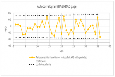
Figure 8. Autocorrelation rk(ξ) of AR (1) with constant Ф, for Baghdad gauge
Figure 9. Autocorrelation rk(ξ) of AR (1) with periodic Ф, for Baghdad gauge
Figure 10. Autocorrelation rk(ξ) of AR (2) with constant Ф, for Baghdad gauge
Suggestion test depending on the rk (ξ) values, the drawing between rk (ξ) and lags (k) produces the correlograms. Correlograms for all models and for all gauges are shown in Figures 8 to 14 with confidence limits that result from Eq. (29). The objective is to find the number of points that lie outside the confidence limits and could be decided upon the better model according to the lower points that lie outside the limits. Firstly, it will compute the points outside the limits using Eqns. (32) to (35) and compare with Correlogram graphics will also be compared with the results from the Portmanteau Lack Test and the results from the AIC Test for all models and for all gages. Through Correlograms from Figures 8 to 11 for the Baghdad gauge, it is very clear that the number of points that lie outside the limits was 1,2,1, and zero for the autocorrelation function of residual of AR1 with constant coefficients, AR1 with constant, and AR2 with periodic, Ф respectively.
Figure 11. Autocorrelation of AR (2) with periodic Ф, for Baghdad gauge
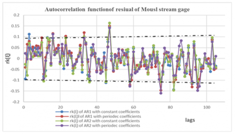
Figure 12. Autocorrelation rk(ξ) for Mousl gauge
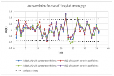
From Eq. (32) through Eq. (35) will compute the number of points that are outside of the limits. The result is illustrated in Table 11, where the AR (2) with periodic Ф is the better model and that is identified with the graphics and also the same conclusion when using the portmanteau lack test and when using the AIC test. Correlograms for Mosul, Kut, and Husaybah were shown in Figures 12 through 14. The results for all gauges when using the suggested test are illustrated in Table 12.
It was seen that there were no suitable models for Mosul gauges because the AC% was less than 95% for all models, so we should try analysis higher-order, anyway. Regarding the AR (2) with periodic Ф model is accepted, this identical with portmanteau lack test and when used AIC test. The better model for Kut gauge is for AR2 with constant. This is identical to the portmanteau lack test and doesn’t match when using the AIC test. So, the suggested test is more reliable if compared with the graphics. Regarding Husaybah gauge from the suggested test, the better model is AR (2) with periodicity. This is Cleary from graphics and similar when used in portmanteau tests and far away when used in AIC tests. Hence, the AIC test gives the AR (1) with constant So the results that are produced from the suggested test are reliable when compared with graphics. This is the proposed statistical method for choosing the best model that depends on the value of the autocorrelation coefficient of the residual rk(ξ) of lag through the acceptance percentage, which represents the percentage of the number of points within the upper and lower limit.
Figure 13. Autocorrelation rk(ξ) for Kut gauge
Table 11. AIC test results
|
Suggest Test |
||||||||
|
Lags |
for AR1 with constant Ф |
for AR1 with periodic Ф |
for AR2 with constant Ф |
for AR2 with periodic Ф |
||||
|
|
Ck or Dk values depending the sign of rk(ξ) |
n’ out |
Ck or Dk values depending the sign of rk(ξ) |
n’ out |
Ck or Dk values depending the sign of rk(ξ) |
n’ out |
Ck or Dk values depending the sign of rk(ξ) |
n’ out |
|
1 |
-0.09801 |
0 |
-0.0688 |
0 |
-0.15627 |
0 |
-0.13153 |
0 |
|
2 |
-0.09404 |
0 |
-0.11427 |
0 |
-0.05353 |
0 |
-0.13332 |
0 |
|
3 |
-0.07811 |
0 |
-0.06913 |
0 |
-0.10461 |
0 |
-0.15424 |
0 |
|
4 |
-0.1009 |
0 |
-0.00448 |
0 |
-0.13489 |
0 |
-0.04307 |
0 |
|
5 |
-0.07168 |
0 |
-0.04318 |
0 |
-0.08819 |
0 |
-0.05005 |
0 |
|
6 |
-0.14957 |
0 |
-0.16021 |
0 |
-0.16296 |
0 |
-0.1419 |
0 |
|
7 |
-0.14587 |
0 |
-0.11144 |
0 |
-0.14398 |
0 |
-0.14399 |
0 |
|
8 |
-0.12079 |
0 |
-0.17456 |
0 |
-0.12275 |
0 |
-0.12389 |
0 |
|
9 |
-0.13353 |
0 |
-0.06689 |
0 |
-0.13414 |
0 |
-0.12951 |
0 |
|
10 |
-0.14708 |
0 |
-0.11976 |
0 |
-0.14664 |
0 |
-0.16413 |
0 |
|
11 |
-0.14421 |
0 |
-0.15096 |
0 |
-0.14262 |
0 |
-0.16648 |
0 |
|
12 |
-0.16917 |
0 |
-0.08649 |
0 |
-0.16079 |
0 |
-0.08819 |
0 |
|
13 |
-0.15271 |
0 |
-0.16022 |
0 |
-0.17567 |
0 |
-0.16851 |
0 |
|
14 |
-0.01201 |
0 |
0.020781 |
1 |
-0.01499 |
0 |
-0.02293 |
0 |
|
15 |
-0.08056 |
0 |
-0.17792 |
0 |
-0.0712 |
0 |
-0.17317 |
0 |
|
16 |
-0.03858 |
0 |
-0.04753 |
0 |
-0.05933 |
0 |
-0.06822 |
0 |
|
17 |
-0.03105 |
0 |
-0.01713 |
0 |
-0.05048 |
0 |
-0.03203 |
0 |
|
18 |
-0.10763 |
0 |
-0.11489 |
0 |
-0.10625 |
0 |
-0.18131 |
0 |
|
19 |
-0.10191 |
0 |
-0.08662 |
0 |
-0.09956 |
0 |
-0.04083 |
0 |
|
20 |
-0.12703 |
0 |
-0.15754 |
0 |
-0.09353 |
0 |
-0.06342 |
0 |
|
21 |
0.108263 |
1 |
0.097073 |
1 |
0.094393 |
1 |
-0.01677 |
0 |
|
22 |
-0.15876 |
0 |
-0.17951 |
0 |
-0.16569 |
0 |
-0.12101 |
0 |
|
23 |
-0.15179 |
0 |
-0.13483 |
0 |
-0.18075 |
0 |
-0.05673 |
0 |
|
24 |
-0.03589 |
0 |
-0.11892 |
0 |
-0.0521 |
0 |
-0.13103 |
0 |
|
25 |
-0.10547 |
0 |
-0.0789 |
0 |
-0.10916 |
0 |
-0.07502 |
0 |
|
26 |
-0.12317 |
0 |
-0.08049 |
0 |
-0.12284 |
0 |
-0.07198 |
0 |
|
27 |
-0.15381 |
0 |
-0.12257 |
0 |
-0.13665 |
0 |
-0.16986 |
0 |
|
28 |
-0.10765 |
0 |
-0.06724 |
0 |
-0.10788 |
0 |
-0.0728 |
0 |
|
29 |
-0.17223 |
0 |
-0.1307 |
0 |
-0.18232 |
0 |
-0.16285 |
0 |
|
30 |
-0.093 |
0 |
-0.07084 |
0 |
-0.09839 |
0 |
-0.09048 |
0 |
|
31 |
-0.08405 |
0 |
-0.14046 |
0 |
-0.09075 |
0 |
-0.14247 |
0 |
|
32 |
-0.19239 |
0 |
-0.14399 |
0 |
-0.18588 |
0 |
-0.19183 |
0 |
|
33 |
-0.16325 |
0 |
-0.17927 |
0 |
-0.1718 |
0 |
-0.16705 |
0 |
|
34 |
-0.07686 |
0 |
-0.04726 |
0 |
-0.06774 |
0 |
-0.07014 |
0 |
|
35 |
-0.08483 |
0 |
-0.03855 |
0 |
-0.0633 |
0 |
-0.04493 |
0 |
|
36 |
-0.06737 |
0 |
-0.08041 |
0 |
-0.05089 |
0 |
-0.03216 |
0 |
|
no. of points outside limits |
1 |
no. of points outside limits |
2 |
no. of points outside limits |
1 |
no. of points outside limits |
0 |
|
|
AC% |
97.22% |
AC% |
94.44% |
AC% |
97.22% |
AC% |
100% |
|
Table 12. Results of suggested test
|
Gages
Models |
AR1 with constant coefficients |
AR1 with periodic coefficients |
AR2 with constant coefficients |
AR2 with periodic coefficients |
|
|
Mosul |
N'out |
9 |
9 |
7 |
6 |
|
AC% |
91.43% |
91.43% |
93.33% |
94.29% |
|
|
Baghdad |
N'out |
1 |
2 |
1 |
0 |
|
AC% |
97.22% |
94.44% |
97.22% |
100% |
|
|
Kut |
N'out |
2 |
2 |
1 |
3 |
|
AC% |
94.44% |
94.44% |
97.22% |
91.67% |
|
|
Husaybah |
N'out |
2 |
3 |
4 |
1 |
|
AC% |
94.44% |
91.67% |
88.89% |
97.22% |
|
Table 13. Results of suggested test
|
Gauges |
Suitable model |
Note |
|
Mosul |
$X_{v, \tau}=\left[-0.142\left(\mu_{\tau}+\sigma_{\tau}\left(\Phi_{1, \tau} Z_{v, \tau-1}+\Phi_{2, \tau} Z_{v, \tau-2}+\sigma_{\varepsilon, \tau} \xi_{v, \tau}\right)\right)+1\right]^{-7.0422}$ |
Values of Φ1, τ, Φ 2, τ, and σε,τ from table (6) and table (8) |
|
Baghdad |
$X_{v, \tau}=\left[-0.691\left(\mu_{\tau}+\sigma_{\tau}\left(\Phi_{1, \tau} Z_{v, \tau-1}+\Phi_{2, \tau} Z_{v, \tau-2}+\sigma_{\varepsilon, \tau} \xi_{v, \tau}\right)\right)+1\right]^{-1.4471}$ |
Values of Φ1, τ, Φ 2, τ, and σε,τ from table (6) and table (8) |
|
Kut |
$X_{t}=\left[-0.263\left(395.24+274.45\left(0.904 Z_{t-1}-0.0121 Z_{t-2}\right.\right.\right.$$\left.\left.\left.+0.2033 \xi_{v, \tau}\right)\right)+1\right]^{-3.8022}$ |
____ |
|
Husaybah |
$X_{v, \tau}=\left[-0.241\left(\mu_{\tau}+\sigma_{\tau}\left(\Phi_{1, \tau} Z_{v, \tau-1}+\Phi_{2, \tau} Z_{v, \tau-2}+\sigma_{\varepsilon, \tau} \xi_{v, \tau}\right)\right)+1\right]^{-4.1493}$ |
Values of Φ1, τ, Φ 2, τ, and σε,τ from table (6) and table (8) |
Figure 14. Autocorrelation rk(ξ) for Husaybah gauge
The current study employs AR (1) and AR (2) with constant and periodic coefficients to analyse data from stations (Mosul, Baghdad, and Kut on the Tigris River, and Husaybah on the Euphrates River) in order to generate data for future years and determine the most appropriate model for each measuring station. The primary purpose of this study was also to offer a new statistical test model for eliciting the number of correlation functions associated with residual points beyond the confidence interval.
The conclusions of this study are divided into two parts, as follows:
[1] Veiga, V.B., Hassan, Q.K., He, J. (2015). Development of flow forecasting models in the Bow River at Calgary, Alberta, Canada. Water, 7(1): 99-115. https://doi.org/10.3390/w7010099
[2] Sathish, S., Babu, S.K. (2017). Stochastic time series analysis of hydrology data for water resources. In IOP Conference Series: Materials Science and Engineering, 263(4): 042140.
[3] Vijayakumar, N., Vennila, S. (2016). A comparative analysis of forecasting reservoir inflow using ARMA model and Holt winters exponential smoothening technique. International Jour. of Innovation in Science and Mathematics, 4(2): 85-90.
[4] Nohani, E. (2015). Forecasting monthly and annual flow rate of Jarrahi River using stochastic model. In Biological Forum, 7(1): 1205-1210. https://doi.org/10.13140/RG.2.2.13933.61929
[5] Adeli, A., Fathi-Moghadam, M., Musavi Jahromi, H. (2014). Using stochastic models to produce artificial time series and inflow prediction: A case study of Talog Dam reservoir, Khuzestan Province. Iran. J. Inter. Bull. Water Resour. Dev, 2(5): 1-13.
[6] Pisarenko, V.F., Lyubushin, A.A., Bolgov, M.V., et al. (2005). Statistical methods for river runoff prediction. Water Resources, 32(2): 115-126. https://doi.org/10.1007/s11268-005-0016-1
[7] Khadr, M. (2016). Forecasting of meteorological drought using Hidden Markov Model (case study: The upper Blue Nile river basin, Ethiopia). Ain Shams Engineering Journal, 7(1): 47-56. https://doi.org/10.1016/j.asej.2015.11.005
[8] Valent, P., Howden, N., Szolgay, J., Komorníková, M. (2011). Analysis of nitrate concentrations using nonlinear time series models. Journal of Hydrology and Hydromechanics, 59(3): 157-170. https://doi.org/10.2478/v10098-011-0013-9
[9] Delgado-Ramos, F., Hervás-Gámez, C. (2018). Simple and low-cost procedure for monthly and yearly streamflow forecasts during the current hydrological year. Water, 10(8): 1038. https://doi.org/10.3390/w10081038
[10] Stojković, M., Prohaska, S., Plavšić, J. (2015). Stochastic structure of annual discharges of large European rivers. Journal of Hydrology and Hydromechanics, 63(1): 63-70.
[11] Saleh, D.K. (2010). Stream Gage Description and Streamflow Statistics for Sites in the Tigris River and Euphrates River Basins, Iraq. U.S. Geological Survey, Reston, Virginia. https://doi.org/10.3133/ds540
[12] Salas, J.D. (1980). Applied Modeling of Hydrologic Time Series. Water Resources Publication.
[13] Box, G.E., Cox, D.R. (1964). An analysis of transformations. Journal of the Royal Statistical Society: Series B (Methodological), 26(2): 211-243.
[14] Maity, R. (2018). Statistical Methods in Hydrology and Hydroclimatology. Springer.
[15] Jayawardena, A.W., Lai, F. (1989). Time series analysis of water quality data in Pearl River, China. Journal of Environmental Engineering, 115(3): 590-607. https://doi.org/10.1061/(ASCE)0733-9372(1989)115:3(590)