Hiranmoy Mandal* | Ujjwal Mondal | Satish Chandra Bera
© 2021 IIETA. This article is published by IIETA and is licensed under the CC BY 4.0 license (http://creativecommons.org/licenses/by/4.0/).
OPEN ACCESS
In the present paper, a modified obstruction free pressure sensor-based flow transducer has been developed using Hall sensors. This technique is a modified version of the earlier inductive method. In this transducer, the fluid pressure in the pipeline is taken as the flow sensing parameter, and various drawbacks of the earlier inductive technique are eliminated. A prototype unit of the transducer is developed and studied in the present work. The transducer consists of two identical C-type Bourdon gauges, each fitted with an identical permanent magnet and Hall sensor assembly to sense the fluid pressure under flow condition and static pressure under no flow condition. The difference between the two Hall sensor outputs is found to vary nonlinearly with flow rate. The mathematical relations describing the working of the prototype unit are derived in the paper. The static characteristic curves of the proposed flow transducer are determined experimentally and reported in the paper. The characteristic curves are found to follow the derived equations to a very good extent with negligible percentage deviation from best-fit nonlinear characteristic.
noncontact flow transducer, Bernoulli’s equation, static pressure, hall sensor, bourdon tube, disk type permanent magnet
Various process fluids used in a process plant are passed through a number of inlet and outlet pipelines. Accurate measurement of the flow rates of these fluids through these pipelines is an essential requirement of the process plant. The flow rate measurement techniques [1-4] may be classified as volume flow rate and mass flow rate. The measurement techniques like obstruction, electromagnetic, ultrasonic, vortex, Hall sensor [2-4], etc. types are the conventional techniques used for volume flow rate measurement. In contrast, the measurement techniques like Coriolis, anemometric types, etc., are conventionally used to measure mass flow rate. Since the volume flow rate measurement methods have a simpler design and lesser cost than the direct mass flow rate measurement techniques, they are used in many applications where the mass flow rate is determined by multiplying the volume flow rate with the density of the fluid. For the incompressible fluids with a constant density, the volume flow meter can be easily converted into the mass flow meter without any calibration but for the other fluids with the density being dependent on pressure, temperature and other factors, the volume flow rate measurement is combined with the density measurement or its correction from pressure and temperature measurements in order to measure the mass flow rate. This difficulty of using a density measurement system or a density correction determination system along with a volume flow meter is avoided in the direct mass flow rate measurement techniques. These conventional volume or mass flow rate measurement techniques being widely used in industry have their relative merits and demerits within certain allowable limits. For example, the obstruction type flow measurement techniques like orifice, venturi etc. may suffer from various problems due to the contact of the sensing element with the process fluid such as reduction of maximum flow capacity of pipeline, use of differential pressure (DP) cell, leakage problem, contact problem etc., but it is still being widely used in industry because of its simple design and low cost. The noncontact techniques like ultrasonic, coriolis etc. are designed to avoid the problems of the contact techniques. The impeller based conventional Hall flow sensor is also a contact type sensor suffering from contact problem of the impeller with the fluid. The main advantage of this flow sensor is that the Hall sensor is not in contact with the fluid and it directly converts the volume flow rate signal into digital signal. Various research works on the flow transducers are still being reported by many groups of researchers. The effect of electrode position in polarization electrode impedance type flow transducer for a conducting liquid has been studied by Bhar et al. [5] and from this study, they have proposed a particular arrangement of electrode position which can provide better sensitivity. Mandal et al. [6] have studied the basic principle of orifice type capacitive flow transducer and the effect of sensing ring position on the sensor capacitance. It has been shown that the sensor capacitance-sensing ring distance product increases linearly with the increase of sensing ring distance from the orifice. Wu et al. [7] have developed a pressure drop prediction model of venturi flow sensor from the drift-flux model and boundary layer theory. From the experimental study, they have shown that the deviation of the experimental value from the model predicted value of pressure drop lies within 15%. A coriolis mass flow meter is a very accurate technique for measurement of mass flow rate of a fluid through a pipe line. Berrocal et al. [8] have proposed a simplified form of the physical model of the coriolis mass flow meter for its use as a volume flow meter. Mua et al. [9] have developed a signal processing technique of ultrasonic flow meter in order to determine the shape of echo signal. It is observed that the echo signal remains almost spindle shape with the increase of flow rate. FPGA and DSP based dual channel ultrasonic flow meter is developed and tested from this echo signal analysis. An accurate computer-based time-of-flight (TOF) measurement algorithm of ultrasonic flowmeter has been developed and tested by Sunol et al. [10] by applying the cross-correlation technique between the transducer output signal and a reference signal. Here, an acoustically forced underdamped oscillator model is developed to produce the reference signal. A modified noncontact Hall sensor and rotameter-based flow transducer is developed by Sinha et al. [11], where the change of the magnetic field of a tiny permanent magnet attached with the rotameter float due to flow is sensed by the Hall sensor mounted on the top of the rotameter. Urbanski et al. [12] have developed a noncontact Hall sensor-based flow transducer where the change of magnetic flux of the rotating permanent magnets attached with the impeller blades is sensed by a Hall sensor. From finite element analysis, it has been shown that the Hall sensor-based flow sensor has better resolution and sensing ability than the conventional turbine type sensors. A flow transducer using Bourdon tube as primary sensing element has been proposed by Marick et al. [13]. In this transducer technique, the decrease of fluid pressure due to increase of flow of a fluid through a pipeline with respect to a static pressure is measured by using two identical Bourdon tubes with identical inductive pick-up coils in which one Bourdon tube system measures the liquid pressure at a given flow and the other identical system measures liquid static pressure at no flow. Li et al. [14] have developed a differential pressure type flow sensor where a V-cone throttling device inserted into the pipeline is used as the primary sensor and the flow rate is virtually displayed by a LabVIEW based monitoring system. Zhang et al. [15] have proposed a flow sensor for measurement of liquid flow rate through microtubes and have shown that the pressure drop across the microtube measured by using micropressure sensor bears a linear relationship with flow rate. The differential pressure type flow measurement systems are found to suffer from a serious drawback due to blockage in the sensing lines.
In the present paper, a modified obstruction free pressure sensor-based flow transducer has been developed using two identical Hall sensors. Two identical Bourdon gauges are used as the pressure sensing elements in the proposed system. The decrease of the pipeline pressure with the increase of a fluid flow rate is the basic principle of the proposed transducer as described by Marick et al. [13]. In this technique, two identical Bourdon pressure gauges are used to measure the pipeline pressure at a given flow rate and the static pressure at no flow. The free tip of each Bourdon gauge is rigidly attached with a tiny permanent magnet in front of a Hall sensor IC mounted on the inside wall of the gauge. The difference between the two similar Hall sensors' outputs is found to vary nonlinearly with the volume flow rate of the fluid. The characteristic equation showing the relation between the transducer output and the volume flow rate is derived in the paper. The developed prototype unit is functionally tested, and the experimental results are reported in the paper. The characteristic curves obtained from the experimental data are found to follow the theoretically derived characteristic equation to a very good extent. The proposed transducer uses stabilized DC source as the excitation source and thus produces the DC output voltage signal. So it eliminates many drawbacks of the existing inductive pick-up type similar transducer [13], such as loss of reliability due to the variation of the magnetic property of the core material, rusting effect of the ferromagnetic wire, the dependence of the transducer output on frequency & waveform of the excitation signal, and requirement of a rectifier & filter unit as an additional component, etc. These defects of the earlier design are avoided in the proposed design.
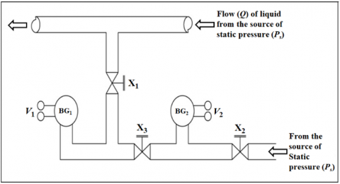
According to Bernoulli's theorem, when a fluid flows through a horizontal pipeline under static pressure, the fluid pressure in the pipeline decreases with the increase of the flow rate. But this decrease of fluid pressure is negligible compared to the static pressure of the fluid at zero flow rate. So in order to utilize this decrease of pressure as a flow sensing parameter, the static pressure must be subtracted from the fluid pressure at a given flow rate. Let us consider two identical C- type Bourdon gauges BG1 and BG2, as shown in Figure 1 used to measure the fluid pressure and the static pressure respectively.
Figure 1. Proposed Bourdon tube type flow measurement system
In Figure 1, the fluid pressure measuring Bourdon gauge (BG1) is connected at a selected point of a horizontal pipeline in the region of no disturbance and the static pressure measuring Bourdon gauge (BG2) is connected to the source of static pressure at a location where there is no flow of the fluid. In the figure, the Bourdon gauge BG1 is connected to the horizontal pipeline through an isolation valve X1 and the Bourdon gauge BG2 is connected to the source of static pressure through an isolation valve X2. The two pressure gauges are isolated from each other through a third isolation valve X3. Under the no flow condition, the pressure in the pipeline becomes equal to the static pressure Ps. So if all the isolation valves are kept open under the no flow condition, then the readings of the Bourdon gauges BG1 and BG2 would be identical and will be equal to static pressure Ps. Under this condition, isolation valve X3 is fully closed keeping the valves X1 and X2 open. Now the process fluid through the horizontal pipeline is allowed to flow at a flow rate Q for which the fluid pressure is P. Under this condition, the Bourdon gauge BG1 will measure the fluid pressure at flow rate Q and the Bourdon gauge BG2 will measure the static pressure Ps at the source.
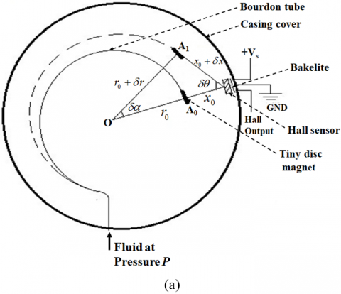
Now the movement of the free tip of each Bourdon pressure gauge is converted into an electrical signal by using a noncontact Hall sensor-based transducer. Two identical transducers are used for the two pressure gauges. Each transducer unit consists of a tiny circular permanent magnet of very small thickness and weight attached with each Bourdon tube's free tip just in front of a Hall sensor IC. The Hall sensor IC is fixed on a Vero-board in a face-to-face location with respect to the magnet. The Vero-board is again fixed with the inside wall of the aluminium casing cover of the pressure gauge through a Bakelite sheet of suitable thickness so that the movement of the free tip of the Bourdon tube may lie in the sensing region of the Hall sensor.
Figure 2. Proposed noncontact Hall sensor-based pressure gauge (a) Schematic diagram (b) Photographic view
Let at the zero-gauge pressure, the straight line joining the Hall sensor IC and the permanent magnet at position A0 is along the radius (OA0) of the Bourdon tube as shown in Figures 2(a) and (b).
Now at a gauge pressure P, the tip of the Bourdon tube rotates through a small angle δα to a position A1 along with the magnet. At this position, the straight line joining the magnet and the Hall sensor IC rotates through a small angle δθ. Let r0 is the Bourdon tube radius at the zero gauge pressure, at which the distance between the magnet and the Hall sensor is x0. Let at the gauge pressure P, the radius of Bourdon tube increases to r0+δr and the gap between the magnet and the Hall sensor IC increases to x0+δx. Since for the small angle of rotation (δα) of the tip of the Bourdon tube, the variations δr, δx, and δθ are also small, so from Figure 2, we may obtain the following approximate Eq. (1).
$\left(r_{0}+\delta r\right) \delta \alpha \approx\left(x_{0}+\delta x\right) \delta \theta$ (1)
Since δr, δx, δα and δθ are very small and δrδα≪r0δα and δxδθ≪x0δθ, so the above Eq. (1) may be approximated as
$r_{0} \delta \alpha \approx x_{0} \delta \theta$ (2)
Let us assume a constant $K_{1}=\frac{r_{0}}{x_{0}}$. Hence the above approximate relation (2) may be written as
$\delta \theta \approx \frac{r_{0}}{x_{0}} \delta \alpha \approx K_{1} \delta \alpha$ (3)
From the principle of Bourdon tube,
$\delta \alpha \propto P=K_{2} P$ (4)
where, K2 is the constant of proportionality.
From (2) and (4), we have,
$\delta \theta=K_{1} \delta \alpha=K_{1} K_{2} P=K_{3} P$ (5)
where, K3= K1K2.
Let at the zero gauge pressure, the magnetic field of the permanent magnet at position A0 acting on the Hall sensor surface be B0 for which the output voltage of the Hall sensor is Vc. Let us also assume that at the gauge pressure P, the position of the permanent magnet is rotated through the small angle (δθ) to a very close position A1, for which the magnetic field acting on the Hall sensor surface becomes Bθ and the Hall sensor output is V1.
Now in the linear region of the Hall sensor characteristic, the Hall sensor output (V1) is linearly related with the magnetic field and can be expressed by the following relation.
$V_{1}=K_{4} B_{\theta}+K_{5}$ (6)
where, K4 and K5 are constants.
From the properties of a permanent magnet, we know that the magnetic field (Bθ) is nonlinearly related with the angle of rotation (δθ) with respect to the Hall sensor. Hence from (6), the Hall sensor output V1 is nonlinearly related with the angle of rotation (δθ). So from the Taylor’s series expansion, V1 can be written as
$V_{1}=V_{c}+\left(\frac{\delta V}{\delta \theta}\right)_{V_{c}} \frac{\delta \theta}{1 !}+\left(\frac{\delta^{2} V}{\delta \theta^{2}}\right)_{V_{c}} \frac{\delta \theta^{2}}{2 !}+\left(\frac{\delta^{3} V}{\delta \theta^{3}}\right)_{V_{c}} \frac{\delta \theta^{3}}{3 !}+\ldots \ldots$ (7)
Now P is the fluid pressure in the pipeline at a flow rate Q and the angle of rotation δα of the tip of the Bourdon tube is very small. Hence from (5), the angle of rotation δθ of the magnet with respect to the Hall sensor is also very small. So neglecting the square and higher order terms in the above equation, we have,
$V_{1} \approx V_{c}+\left(\frac{\delta V}{\delta \theta}\right)_{V_{c}} \delta \theta$
or, $V_{1}=V_{c}+a_{1} \delta \theta$ (8)
where, $\quad a_{1}=\left(\frac{\delta V}{\delta \theta}\right)_{V_{c}}$ (9)
From (5) and (8), we have,
$V_{1}=V_{c}+a_{1} K_{3} P=V_{c}+a_{2} P$ (10)
where, a2=a1K3.
Now from the Bernoulli’s equation, the fluid pressure P decreases nonlinearly with the increase of flow rate. Hence from the above equation, the Hall sensor output V1 for the Bourdon gauge BG1 decreases nonlinearly with the increase of the flow rate of the fluid through the pipeline. But in case of the other Bourdon gauge BG2, there is no flow of fluid since this gauge connected to the source of driving pressure at a point where there is no flow of the fluid. So BG2 measures the static pressure (Ps) of the fluid which may be assumed to be constant. Hence from (10), the Hall sensor output V2 for the Bourdon gauge BG2 at a static pressure P=Ps may be given by
$V_{2}=V_{c}+a_{2} P_{s}$ (11)
Let under the no flow condition, the isolation valves X1, X2, and X3 are open so that the transducer outputs in both the pressure gauges are identical. Under this condition, the isolation valve X3 is fully closed and the fluid is allowed to flow through the pipeline with the valves X1 and X2 fully open. So the pressure of the fluid will decrease and the output (V1) of the Hall sensor in BG1 will decrease.
Following the similar analysis as stated in [13], the reduced fluid pressure P' due to flow is obtained from the Bernoulli’s equation and the resulting vacuum pressure P'' inside the Bourdon tube are given by the following Eqns. (12) and (13) respectively.
$\frac{Q^{2}}{2 A^{2}}+\frac{P^{\prime}}{\rho}=K_{6}$ (12)
$P^{\prime \prime}=K_{7} Q+K_{8}$ (13)
where, K6, K7, and K8 are Constants.
Hence the effective pressure P inside the Bourdon tube is given by
$P=P^{\prime}-P^{\prime \prime}=\rho K_{6}-\frac{\rho Q^{2}}{2 A^{2}}-K_{7} Q-K_{8}=K_{9}-K_{7} Q-K_{10} Q^{2}$ (14)
where, $\quad K_{9}=\rho K_{6}-K_{8}$ and $K_{10}=\frac{\rho}{2 A^{2}}$ (15)
where, ρ= Density of the fluid, A= Area of cross section of pipeline, Q= Volume flow rate of the fluid.
Combining (10) and (14), we have,
$V_{1}=V_{c}+a_{2}\left(K_{9}-K_{7} Q-K_{10} Q^{2}\right)=V_{c}+a_{3}-b_{1} Q-c_{1} Q^{2}$ (16)
where, $a_{3}=a_{2} K_{9}, b_{1}=a_{2} K_{7}$ and $c_{1}=a_{2} K_{10}$ (17)
Now in (12), if we put Q=0 then P' becomes equal to static pressure Ps.
i.e., $\frac{P_{s}}{\rho}=K_{6}$ (18)
Hence, from (15), (17) and (18) we have,
$a_{3}=a_{2} K_{9}=a_{2}\left(\rho K_{6}-K_{8}\right)=a_{2}\left(P_{s}-K_{8}\right)$ (19)
Combining (16) and (19), we have,
$V_{1}=V_{c}+a_{2} P_{s}-a_{2} K_{8}-b_{1} Q-c_{1} Q^{2}$ (20)
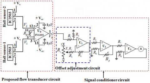
Hence from (11) and (20), it is observed that the effect of the static pressure is eliminated if we take the difference between the output signals V1 and V2 of the two Hall sensors. This difference is obtained by using an instrumentation amplifier IC (U0) as shown in Figure 3.
Figure 3. The proposed Hall sensor-based flow transducer circuit with signal conditioner of the transmitting part
In Figure 3, the Hall sensor-1 and Hall sensor-2 are two identical Hall sensor ICs installed in the pressure gauges BG1 and BG2 respectively as shown in Figure 1. Both the Hall sensors are supplied from the same stabilized DC source +Vs. As stated earlier, the difference between the Hall sensor output voltage signals (V1 & V2) is amplified by using the instrumentation amplifier IC.
Let us select a gain KI of the instrumentation amplifier by selecting a suitable value of gain adjustment potentiometer Rg shown in Figure 3. So from (11) and (20), the output V0 of the proposed transducer circuit shown in Figure 3, may be given by,
$\begin{aligned} V_{0} &=K_{I}\left(V_{2}-V_{1}\right) \\ &=K_{I}\left[\left(V_{c}+a_{2} P_{s}\right)-\left(V_{c}+a_{2} P_{s}-a_{2} K_{8}-b_{1} Q-c_{1} Q^{2}\right)\right] \end{aligned}$ (21)
or, $V_{0}=a+b Q+c Q^{2}$ (22)
where, $a=a_{2} K_{I} K_{8}=$ offset, $b=b_{1} K_{I}$ and $c=c_{1} K_{I}$ (23)
Thus the transducer output increases nonlinearly with increase of flow rate.
It may be mentioned here that the instrumentation amplifier shown in Figure 3 is selected in order to reduce the effect of noise and to have very high signal to noise ratio at the transducer output. Moreover, very high input impedance of the instrumentation amplifier IC draws very negligible current from the outputs of the Hall sensors so that each Hall sensor output may be free from loading effect error. Since the two Hall sensors are identical and are kept in the same atmospheric temperatures inside the two Bourdon gauges so the changes of their output voltages V1 and V2 due to atmospheric temperature variation will be identical and will cancel each other. Again, the temperature sensitivity of a Hall sensor is also dependent on temperature. So a gain drift error of each Hall sensor due to the effect of temperature may be produced in the transducer output. But since the two identical Hall sensors are sensing the pressure of the same liquid at the same atmospheric temperature, the gain drift error due to temperature may be assumed to be identical for both the Hall sensors and cancel each other in the instrumentation amplifier circuit. Hence the instrumentation amplifier's output V0 will be free from the measurement error due to the variation of atmospheric temperature.
The output signal of the proposed transducer follows the nonlinear characteristic Eq. (22). This nonlinear characteristic can be easily linearized by using hardware-based or software-based piece wise linearization techniques. Here the constant ‘a’ in this characteristic equation denotes the transducer output at zero flow rate. So, it denotes the offset voltage of the transducer. This can be easily eliminated by using an offset adjustment circuit as shown in the in the signal conditioner section of the flow transmitting part of Figure 3. In the present paper, only the transducer part has been studied to avoid the unnecessary increase in the paper's length.
The design of a prototype flow transducer unit is developed using two identical C-type Bourdon tubes, as shown in Figure 1 with tap water acting as the process fluid. Thus the design of the whole transducer unit consists of the selection of the main pipeline, connector lines, isolation valves, C-type Bourdon gauges with magnet and Hall sensor assemblies. A prototype unit of the flow transducer is designed using C-type Bourdon gauges with magnet and Hall sensor assemblies by selecting them with the designed parameters as shown in Table 1.
Table 1. Design parameters
|
Sl. No. |
Item selected in the design |
Item parameter |
Selection criteria |
|
1 |
Identical C-type Bourdon pressure gauges (2 Numbers) |
Pressure measuring range (0-1) kg/cm2 or (0-100) kPa, dial diameter 0.15-meter, C-type Bourdon tube diameter 0.113 meter |
C-type Bourdon tubes with high resolution are selected because they are simple, reliable & less costly and the available static pressure is small along with the small change of pipeline pressure with flow rate. |
|
2 |
Identical Permanent magnets (2 Numbers) |
Circular disc type with thickness 2 mm, diameter 10 mm, weight- 2.5 gm, material – Alnico |
The permanent magnets are made of alnico. From the manufacturer’s data manual, the selected magnet material is found to have high values of coercivity (0.07 T) and remanence (1.35 T) with very good resistance to temperature effect up to 525℃ and can retain the stable magnetic properties with high resistance to corrosion. |
|
3 |
Identical Hall sensor ICs (2 Numbers) |
UGN3503U |
Hall sensors are selected as IC UGN3503U due to its following good performance characteristics (as per datasheet): Linear zone for magnetic field in the range (-900 to +900) G, High sensitivity (0.75 to 1.75) mV/G, Operating temperature range: -20℃ to +85℃. |
|
4 |
Instrumentation Amplifier |
INA101 (U0) |
The instrumentation amplifier is selected as the very low noise IC INA101 with the following parameters (as per datasheet) favorable for its use as a low signal amplifier: Low drift (0.25µV/℃ max), Low offset voltage (25µV max), Low nonlinearity (0.002%), Low noise ($13 \mathrm{nV} / \sqrt{\mathrm{Hz}}$), High CMRR (106dB at 60Hz), High input impedance (1010 Ω.) |
|
5 |
Potentiometers |
Metal film linear, 1 watt, with ±5% tolerances having the values: Rg: 0–22 KΩ. |
-------------- |
|
6 |
Non-electrolytic capacitors (2 Numbers) |
Ceramic capacitor, 1 µF, 1000 Volt |
-------------- |
|
7 |
Isolation valves (4 Numbers) |
GI ball valves |
-------------- |
|
8 |
Pipelines and connectors |
PVC pipelines and galvanized iron (GI) connectors |
-------------- |
The main pipeline is selected as uniform polyvinyl chloride (PVC) pipe of internal diameter 25 mm. It is rigidly fixed in horizontal position on a rigid support at the ground level of the laboratory and is connected with a constant level overhead tank through an isolation valve. The other end of the horizontal pipeline is connected with a vertically mounted rotameter and the outlet of the rotameter is connected to the underground reservoir tank through a PVC pipe of the same diameter as the main pipe. For connection of the pressure gauges, galvanized iron (GI) connector pipes and PVC tubes each with 12 mm internal diameter and suitable length are used in the design of the prototype unit of the transducer. Commercially available ball valves are selected for the isolation valves. The permanent magnets attached with the free tips of the two Bourdon gauges are selected as tiny strong circular permanent magnets each with identical pole strength having diameter 10 mm, thickness 2 mm, and weight 2.5 gm.
In each pressure gauge, a thin piece of a Vero-board mounted with a Hall sensor IC is fastened on the inside surface of the pressure gauge cover through Bakelite sheets of suitable sizes using brass screws so that the Hall sensor sensing surface may remain just in front of the tiny magnet, as shown in Figure 2(b). The thickness of the Bakelite sheet is selected in order to bring the gap length between magnet and Hall sensor within the linear sensing region. From the experimental study of the selected magnet and Hall sensor system, it is observed that the Hall sensor output varies almost linearly when the given magnet is brought within a distance between 10 mm and 18 mm from the Hall sensor. In the proposed technique, this distance is selected as 15 mm by means of Bakelite sheet of suitable thickness so that at maximum pressure, the movement of the tip of the Bourdon gauge towards the Hall sensor may remain within a distance greater than 10 mm.
Each Hall sensor IC is fixed with a Vero-board through the soldered joints avoiding any dry soldering. Three lead wires from the three pins of each Hall sensor IC are brought out through a small opening in the pressure gauge casing and connected with the instrumentation amplifier IC fixed on a second Vero-board outside the pressure gauge. The instrumentation amplifier IC and each Hall sensor IC are supplied from a stabilized 30 VA voltage regulator unit giving ripple free stabilized DC supply at 0 Volt, +15 Volt, -15 Volt, and +5 Volt. Each Hall sensor IC is supplied from the same +5 Volt source and the instrumentation amplifier is supplied from ±15 Volt source. The instrumentation amplifier IC INA101 with minimum gain $\left(K_{I}=1+\frac{40 \mathrm{k} \Omega}{R_{g}}\right)$ is selected as 5 by selecting the gain adjustment potentiometer (Rg) as shown in Figure 3 as 1 watt, 10 kΩ metal film potentiometer.
The experiment was carried out with an experimental setup as schematically shown in Figure 4. In Figure 4, the overhead tank is supplied from an underground reservoir tank by an ac motor-driven pump. The supply voltage of the pump is adjusted using a variac so that the output flow rate (Q1) of water to the overhead tank is always greater than the maximum flow rate of water through the horizontal test pipeline and the excess water is exhausted through an exhaust pipeline back to the underground tank. Thus the level in the overhead tank is maintained constant throughout the experiment. The horizontal main pipeline in the ground level of the laboratory fixed on a rigid support is connected with the overhead tank through an isolation valve X4 as shown in Figure 4.
The flow rate of water is measured by a pre-calibrated rotameter and the water passing through the rotameter is sent back to the underground tank through a PVC pipe. The bottom of the overhead tank is always at zero flow condition so that the Bourdon gauge BG2 with isolation valve X2 open measures the static pressure in the pipeline which is maintained constant throughout the experiment since the level of the water in the overhead tank is always constant. With the isolation valve X3 fully closed and X1 open, the Bourdon gauge BG1 measures the pressure of the flowing fluid in the horizontal test pipeline. The Hall sensor-based sensing systems mounted in the Bourdon gauges BG1 and BG2 convert the respective pressure signals into voltage signals V1 and V2. At zero flow condition with flow adjustment valve X4 closed, the three isolation valves X1, X2, and X3 were open so that the outputs of pressure gauges BG1 and BG2 were equal. Under this condition, the isolation valve X3 was made fully closed and the flow rate of water through the test pipeline was increased in steps by adjusting the valve X4. At each step, the transducer output (V0) was measured by a 4½-digit digital multimeter and the corresponding flow rate was obtained from the pre-calibrated rotameter. The rotameter was calibrated by the direct water collection method and was found to have a measurement error within ±0.5%.
Figure 4. Schematic diagram of an experimental set-up
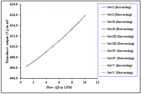
Figure 5. Static characteristic curves of the proposed flow transducer observed in ten repetitions
The experiment was repeated ten times in both increasing and decreasing modes at different times on different dates under the laboratory's same environmental condition. The static characteristic curves of the proposed flow transducer were drawn by plotting the transducer output against the flow rate, as shown in Figure 5.
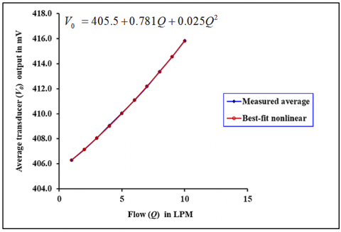
As shown in Figure 5, the average values of transducer output at different flow rates were determined from the measured data obtained in ten repetitions. It is shown that vertical coordinates are in mV in Figure 5 and horizontal units are in liter per minute (LPM). The average static characteristic curve of the proposed transducer was then drawn by plotting the average transducer output against flow rate, as shown in Figure 6. From this average static characteristic curve, the best-fit curve along with the best-fit characteristic equation is drawn using the Microsoft Excel program as shown in the same figure. In Figure 6, vertical coordinates are in mV and horizontal units are in LPM.
Figure 6. Average static characteristic curve of the proposed flow transducer along with best-fit nonlinear characteristic
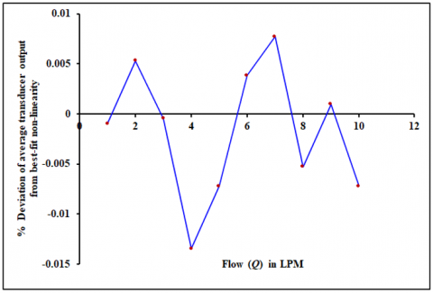
The corresponding percentage deviations of the measured data from best-fit nonlinear characteristic at different flow rates were determined using the Microsoft Excel program, as shown in Figure 7. In Figure 7, the vertical coordinates are in percentage deviation or percentage error of average transducer output voltage from the respective best fit nonlinear characteristic voltage as shown in Figure 6. The horizontal units are in LPM in Figure 7.
Figure 7. Percentage deviation curve from best-fit characteristic of the proposed flow transducer
From the measured data obtained from ten repetitions, the standard deviation (σ) of the experimental data at each flow rate was determined using the Microsoft Excel program. From this value of the standard deviation, the repeatability (r) of data at each flow rate was determined by using the following formula recommended by the American Society for Testing and Materials (ASTM) [16] $r=2 \sqrt{2} \sigma_{r}=2 \sqrt{2} \frac{\sigma}{\bar{X}_{\max }} \times 100 \%$ of maximum range, where σr is the relative standard deviation and $\bar{X}_{\max }$= Maximum average value of the measured data obtained in ten repetitions. The repeatability curve of the proposed transducer was then drawn by plotting the repeatability against the flow rate, as shown in Figure 8. In Figure 8, the vertical coordinates are in percentage repeatability of transducer output in the percentage of the maximum range of the transducer, whereas horizontal coordinates are in LPM.
Figure 8. Repeatability curve of the proposed flow transducer curve obtained from measured data in ten repetitions
The static characteristic curves of the proposed transducer shown in Figure 5 are drawn from the measured data obtained in ten repetitions of the experiment under the same environment of air-conditioned laboratory maintained at 25℃ at different dates and times throughout a year. Almost identical curves reveal good reliability of the transducer. From the average static characteristic curve and the best-fit curve shown in Figure 6, the best-fit characteristic equation of the proposed flow transducer is given by V0=405.5+0.781Q+0.025Q2, which is similar to the derived Eq. (22) with the offset constant $' a^{\prime}$= 405.5 mV, and the other constants 'b'= 0.781 mV/LPM, and 'c'=0.025 mV/(LPM)2. The typical signal conditioner circuit shown in Figure 3 may be used to convert the transducer output into standard current signal of a flow transmitter. The low percentage deviation from the best-fit curve shown in Figure 7 indicates that the average characteristic curve follows the derived Eq. (22) to a very good extent. The repeatability curve in Figure 8 shows very small standard deviation and very good repeatability of the proposed transducer.
The tip of each metallic Bourdon tube attached with the tiny permanent magnet and the noncontact Hall sensor IC being exposed to atmosphere are all maintained at atmospheric temperature. So the liquid temperature has little effect on the strength of the permanent magnet and the Hall sensor output in each pressure gauge. Long time stability of the magnetic strength of the alnico made permanent magnet along with stable DC supply voltage ensure good stability and longevity of the proposed transducer.
The two Hall sensor ICs being supplied from the same stabilized DC source produce identical output voltage variations due to the fluctuation of the supply voltage, which are cancelled out in the instrumentation amplifier circuit. Small weight and small size of the tiny permanent magnet has little effect on the free movement of the tip of the Bourdon tube having high mechanical strength.
The differential pressure (DP) cell type measurement technique in obstruction flow meter may suffer from a serious blockage problem due to storing of gas bubble in the sensing line. It may also suffer from various other problems such as mounting problem, leakage problem, contact problem. In addition to these problems it also may arise from much more complicated and costly design of the DP cell system compared to the proposed measuring system. The mounting of Bourdon gauges in the proposed measuring system is also much simpler with much less maintenance problems compared to the DP cell type system.
Since in most of the flow applications, the flow through a pipeline occurs from a static pressure source like overhead tank, pump, pressure vessel etc. so the region of zero flow condition may be easily available. The additional cost on piping work for the connection of static pressure sensing pressure gauge may be reduced by selecting the mounting location nearer to the static pressure source. Moreover, the presence of no obstruction in the pipeline helps in obtaining the maximum flowing capacity for a given static pressure. Hence the proposed technique with very simple design may be assumed to have good acceptability in industry.
The larger diameter C-type Bourdon tubes with small range and high resolution are selected for the proposed design because they are less costly and the available static pressure is small along with the small change of pipeline pressure with flow rate. However, for higher static pressure, the other pressure sensors with better resolution may be used such as diaphragm, bellows etc. combined with secondary sensing elements like strain gauge, piezo-resistance, piezo-electric element, and sputtered thin film element etc.
The value of the offset voltage (a) shown in Eq. (22) is experimentally found to be about 405.5 mV as shown in Figure 6 whereas the change of the transducer output for change of flow rate from 0-10 LPM is about 10 mV. This high value of offset may be due to the mismatch between the two Bourdon tube-Hall sensor based sensing systems. So in the transmitter circuit this offset is eliminated by adjusting the offset adjustment potentiometer so that the transducer output is zero at zero flow rate.
The novelty of the proposed flow transducer is that it has successfully modified the existing inductive pick-up type transducer described in ref. [13] by eliminating its drawbacks such as requirement of stabilized sinusoidal ac excitation signal, rectifier & filter unit, error due to variation of frequency & waveform of the excitation signal, stray capacitance effect, rusting effect, and mounting instability of ferromagnetic wire, etc. The derived performance equation of the proposed flow transducer is supported by the experimental results to a very good extent with excellent repeatability and very small percentage error.
From a comparative study of the proposed transducer with some of the other volume flow rate transducer as given in the following Table 2, it may be concluded that the proposed flow transducer may be assumed to have good industrial acceptability.
Table 2. Comparative study of the proposed flow transducer with some other volume flow rate transducers
|
Parameters |
Types of volume flow rate transducer |
||||||
|
Orifice [2] |
Vortex shedding [2] |
Electro-magnetic [2] |
Elbow taps [2] |
Inductive pick-up [13] |
Proposed transducer |
Inference |
|
|
Excitation source |
AC/DC |
AC |
AC/DC |
AC |
AC |
DC |
Compared with other sensors, the proposed sensor is more comfortable to design and less costly. It is very quickly reparable with ambient temperature error, simple assembly technique, comparable accuracy, reliability, repeatability & more longevity. |
|
Stray capacitance error |
Present |
Present |
Present |
Present |
Present |
Absent |
|
|
Assembling technique |
Simple |
Complicated |
Complicated |
Complicated |
Simple |
Very simple |
|
|
Cost |
Costly |
Costly |
Costly |
Costly |
Less costly |
Least costly |
|
|
Rectifier & filter |
Required for AC |
Required |
Required for AC |
Required |
Required |
Not required |
|
|
Pressure loss across sensor [2] |
High |
High |
High |
None |
None |
None |
|
|
Atmospheric temperature Compensation |
Required |
Required |
Required |
Required |
Required |
Not required |
|
|
Longevity |
High |
High |
High |
High |
Not so high |
Very high |
|
|
Sensor repairing |
Possible & easy |
Possible |
Possible |
Possible & easy |
Possible & easy |
Possible & very easy |
|
|
Primary- secondary contact |
Contact type |
Contact type |
Contact type |
Contact type |
Noncontact type |
Noncontact type |
|
|
Accuracy (% of full scale) [2] |
0.5-2% |
0.5-1.5% |
0.5-2% |
5-10% |
< 1% |
< 1% |
|
The authors are thankful to the Department of Applied Physics, Instrumentation Engineering, University of Calcutta and Academy of Technology, Hooghly for providing the facilities to carry out the work in the present investigation.
[1] Doeblin, E.O. (1990). Measurement System Application and Design (4th ed.). New York, USA: McGraw-Hill.
[2] Liptak, B.G. (1999). Process Measurement and Analysis (3rd ed.). Oxford, U.K.: Butterworth Heinman.
[3] Hall Effect Sensing and Application. Sensing and Control, Honeywell Inc. Freeport, Illinois, USA. https://sensing.honeywell.com/hallbook.pdf.
[4] Ramsden, E. (2011). Hall-Effect Sensors: Theory and Application (2nd ed.). Oxford, U.K.: Newnes.
[5] Bhar, I., Mandal, N. (2020). Effect of position of electrodes in polarization type flowmeter: analysis and experimental evaluation. IEEE Transactions on Instrumentation and Measurement, 69(6): 3061-3069. https://doi.org/10.1109/TIM.2019.2931527
[6] Mandal, H., Bera, S.K., Sadhu, P.K., Bera, S.C. (2020). Further study of the sensing ring position on the orifice-type capacitive flow sensor. IEEE Transactions on Instrumentation and Measurement, 69(4): 1812-1820. https://doi.org/10.1109/TIM.2019.2913060
[7] Wu, H., Xu, Y., Xiong, X., Mamat, E., Wang, J., Zhang, T. (2020). Prediction of pressure drop in Venturi based on drift-flux model and boundary layer theory. Flow Measurement and Instrumentation, 71: 101673. https://doi.org/10.1016/j.flowmeasinst.2019.101673
[8] Berrocal, A.G, Montalvo, C., Carmona, P., Blazquez, J. (2019). The Coriolis mass flow meter as a volume meter for the custody transfer in liquid hydrocarbons logistics. ISA Transactions, 90: 311-318. https://doi.org/10.1016/j.isatra.2019.01.007
[9] Mua, L.B., Xu, K.J., Liu, B., Tian, L., Liang, L.P. (2019). Echo signal envelope fitting based signal processing methods for ultrasonic gas flow-meter. ISA Transactions, 89: 233-244. https://doi.org/10.1016/j.isatra.2018.12.035
[10] Sunol, F., Ochoa, D.A., Garcia, J.E. (2019). High-precision time-of-flight determination algorithm for ultrasonic flow measurement. IEEE Transactions on Instrumentation and Measurement, 68(8): 2724-2732. https://doi.org/10.1109/TIM.2018.2869263
[11] Sinha, S., Banerjee, D., Mandal, N., Sarkar, R., Bera, S.C. (2015). Design and implementation of real-time flow measurement system using hall probe sensor and PC-based SCADA. IEEE Sensors Journal, 15(10): 5592-5600. https://doi.org/10.1109/JSEN.2015.2442651
[12] Urbanski, M., Nowicki, M., Szewczyk, R., Winiarski W. (2015). Flowmeter converter based on hall effect sensor. Progress in Automation, Robotics and Measuring Techniques. Advances in Intelligent Systems and Computing, Springer, 352: 265-276. https://doi.org/10.1007/978-3-319-15835-8_29
[13] Marick, S., Bera, S.K., Bera, S.C. (2014). A modified technique of flow transducer using bourdon tube as primary sensing element. IEEE Sensors Journal, 14(9): 3033-3039. https://doi.org/10.1109/JSEN.2014.2322199
[14] Li, F., Dong, F., Zhang, F. (2011). A measurement system of cone meter differential pressure based on LabVIEW. IEEE Conference on 30th Chinese Control, Yantai, China, pp. 5815-5819.
[15] Zhang, X., Coupland, P., Fletcher, P.D.I., Haswell, S.J. (2009). Monitoring of liquid flow through microtubes using a micropressure sensor. Chemical Engineering Research and Design, 87(1): 19-24. https://doi.org/10.1016/j.cherd.2008.06.007
[16] Standard Guide for Conducting a Repeatability and Reproducibility Study on Test Equipment for Nondestructive Testing (2004). Standard ASTM F1469–11. https://www.astm.org/Standards/F1469.htm.