Dapeng Wen | Xiyin Liang* | Maogen Su | Meng Wu | Ruilin Chen | Tianchen Zhang
© 2021 IIETA. This article is published by IIETA and is licensed under the CC BY 4.0 license (http://creativecommons.org/licenses/by/4.0/).
OPEN ACCESS
Aiming at the problems that the weak current signal circuit is susceptible to noise interference and leakage current at the input terminal affects the measurement accuracy, a weak current measurement error correction scheme based on the combination of wavelet threshold denoising and generalized regression neural network (GRNN) was proposed. The scheme was applied to the error correction of multi-channel weak current measurement system based on the ADAS1134 chip: the wavelet threshold denoising was used to preprocess the original current data measured by the system and the current measurement value was corrected after the system measurement error correction model established with GRNN was constructed. Compared with the correction method based on least square method and back propagation neural network (BPNN), this method has many advantages such as high accuracy, anti-interference ability and strong generalization ability. The experimental results showed that RMSE=0.0911 nA, MAE=0.0354 nA, and MAPE=0.0078%, without increasing the complexity of the measurement circuit, which achieved the purpose of correcting the measurement error of the weak current measurement system.
BPNN, GRNN, measurement error, weak current, wavelet denoising
In many fields such as radiation measurement technology, space particle detection technology, medical CT imaging technology, heavy ion beam therapy technology, etc., it is necessary to accurately measure weak current of the nA order or less [1-5]. Weak current measurement is vulnerable to some factors (e.g., noise interference, temperature drift and leakage current at input) affecting the measurement accuracy [6, 7], which influences the overall performance of the system. Therefore, in order to improve the overall performance of the system using the weak current detection technology, it is essential to improve the measurement accuracy of the weak current.
At present, the weak current measurement methods mainly include the current-to-voltage method and the current-to-frequency method [7-9]. The current-to-voltage method comprises the capacitance integration method and the feedback resistance method. The capacitance integration method to measure weak current is affected by the capacitance value. When the capacitance value is too large, the sensitivity of the measurement is reduced, and the real-time performance is bad, which is suitable for intermittent measurement of weak current signals [7]. The noise of the capacitance integration method mainly comes from thermal noise and amplifier active noise [10]. Also, the feedback resistance method is mostly composed of feedback resistance and operational amplifier, so it can realize continuous real-time measurement of weak current signals. The feedback resistance method requires a larger resistance, but the large resistance is easily influenced by temperature. The noise of this method mainly comes from the feedback resistance and the operational amplifier [9]. The structure of the current-to-frequency method is complicated, and the circuit is difficult to debug. Not only does the insufficiency of the measurement circuit itself can cause the measurement noise, but also the PCB material of the circuit board and the wiring installation way of the input terminal will lead to leakage current at input in the weak current measurement system, resulting in measurement errors in the system [11, 12]. So far, the hardware conditions of weak current measurement have been improved to reduce the influence of noise, temperature, leakage current at input and other factors on the accuracy of weak current measurement. For example, Kim et al. [9] used the correlated double sampling (CDS) technique and a low-pass filter that can change the bandwidth according to the frequency of the input signal to improve the noise performance of the synchronous capacitance integration method used in weak current measurement systems. Guo et al. [7] employed the ADA4430 chip to design a weak current measurement circuit that can measure uA ~ pA. Specially, the ADA4430 chip has an ultra-low bias current electrometer op amp and an integrated guard ring buffer used to isolate input pins to prevent PCB board leakage current. Li and Hao et al. [11, 12] proposed that in the design of weak current measurement circuit, some measures should be taken to reduce noise interference and temperature drift, such as decoupling filter of power supply, removing balance resistance at input terminal of operational amplifier, reducing power consumption of operational amplifier and using partial feedback to reduce feedback resistance and output filter. For the process structure, in order to reduce noise interference and leakage current at input, the steps can be taken are: choose a PCB with high insulation strength and low leakage current; take shielded cable as the input signal line fixed and hung by a PTFE material bracket in the air; shield low current amplifiers by metal boxes.
Improving the hardware conditions of the weak current measurement system can better enhance the weak current’s measurement accuracy, but it will increase the complexity and cost of the circuit system design. Thus, a software algorithm method was proposed in this work to correct the measurement error of weak current mainly caused by noise and leakage current at input. In this paper, the wavelet denoising method is used to preprocess the collected original current data, and a soft threshold is used for denoising. By comparing the effect of wavelet threshold denoising on the original current data by using different wavelet basis functions and different decomposition levels, using the db5 wavelet basis function to denoise the original current data with 4 levels has the best denoising effect. Therefore, in this paper, wavelet threshold denoising uses db5 wavelet basis function to decompose the original current data in 4 levels. Then, GRNN is used to establish a system measurement error correction model to correct the system measurement error, and the grid search method is used to optimize the smoothing factor parameters of GRNN. By establishing two correction models of least square method and BPNN respectively, and comparing experiments with the GRNN correction model, the experimental results show that the GRNN correction model has a better correction effect. The method presented in this paper was used for measuring error correction in the current acquisition system designed with the ADAS1134 chip. And the system measures weak current using the capacitance integration method. After verification on the experimental system, a conclusion could be come to that the proposed method can correct very well the measurement error of weak current measurement system and the accuracy of measurement has been improved by virtue of software algorithm.
2.1 Wavelet denoising algorithm
Wavelets are orthogonal bases of finite length that can be used to represent a time series into a time-scale domain at different resolutions [13]. In this paper, the denoising capabilities of wavelet transforms were used to preprocess the weak current data to improve the error correction capabilities of the neural network model. The method of wavelet denoising on the basis of threshold processing, initialized by Dohono, can estimate the threshold value through wavelet transform coefficient and reconstruct signals with the retained wavelet coefficient [14]. The basic model of wavelet denoising can be set as:
$s(t)=f(t)+\delta n(t)$ (1)
Among them: s(t) is the signal containing noise; f(t) is the original signal; n(t) is the noise signal, δ is the noise intensity. Wavelet threshold denoising can be performed in the following 3 steps [15]:
(1) Perform wavelet transform on the signal with noise: selecting a wavelet base, determining the decomposition scale N, and then performing N-level wavelet decomposition on the signal s(t) to obtain wavelet decomposition coefficients W;
(2) Perform threshold processing on wavelet coefficient: calculating the wavelet threshold λ, selecting the appropriate threshold function(soft threshold or hard threshold), and quantizing the wavelet coefficients to obtain new wavelet coefficients Wλ;
(3) Reconstruct the signal: performing wavelet inverse transformation on the obtained wavelet coefficients Wλ to obtain the denoised signal.
The soft threshold function was obtained by improving the hard threshold function, and the denoising effect was smoother than that of the hard threshold function. The definition of the soft threshold function used in this study is shown in Eq. (2) [16]:
${{\overline{\text{w}}}_{j,k}}=\left\{ \begin{matrix} sgn ({{w}_{j,k}})({{w}_{j,k}}-\lambda ),\left| {{w}_{j,k}} \right|\text{ }\lambda \\ 0,\left| {{w}_{j,k}} \right|\text{ }\lambda \\\end{matrix} \right.$ (2)
In the formula, sgn(⋅) is sign function, $w_{j, k}$ and $\bar{w}_{j, k}$ represent the wavelet coefficients before and after the denoising process, respectively, and λ represents the threshold. General threshold adopted in this paper is as follows:
$\lambda =\delta \sqrt{2\ln X}$ (3)
Here X is signal length and $\delta=\frac{\operatorname{median}\left(\left|w_{j, k}\right|\right)}{0.6745}$ [17].
So far, there has not been mature theory to guide how to choose wavelet basis functions. However, in many practices of wavelet analysis, some relatively effective experience guidance can be obtained. To illustrate, for the processing of digital signals, Haar or Daubechies wavelet basis functions can often get better processing results, and Daubechies wavelet is an orthogonal wavelet function with compact support created by the famous wavelet scholar, Ingrid Daubechies [18]. Daubechies series wavelets are called dbN for short. Therefore, only those wavelet basis functions are considered in this paper. The determination of the best wavelet basis function and decomposition levels is discussed in Section 4.1.
In this paper, the wavelet threshold denoising method was used to preprocess the weak current signal sampling data, which can improve the validity and completeness of the data to a certain extent, thereby improving the generalization ability and accuracy of model prediction.
2.2 GRNN model
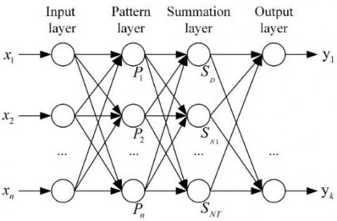
Generalized Regression Neural Network (GRNN) was put forward by American scholar Donald F. Specht in 1991. It owns strong nonlinear mapping ability, flexible network structure, as well as high fault tolerance and robustness, which is suitable for solving nonlinear problems [19]. In contrast with other iterative networks, GRNN possesses less training time (See Figure 1) [20].
Figure 1. The structure of general regression neural network (GRNN)
The structure of GRNN model contains four layers, that is, input layer, pattern layer, summation layer and output layer respectively [21]. In this structure, the input vector $X=\left[x_{1}, x_{2}, \ldots, x_{n}\right]^{T}$, the output vector $Y=\left[y_{1}, y_{2}, \ldots, y_{k}\right]^{T}$, $P_{i}=\exp \left[-\frac{\left(X-X_{i}\right)^{T}\left(X-X_{i}\right)}{2 \sigma^{2}}\right](i=1,2, \ldots, n) \quad, \quad S_{D}=\sum_{i=1}^{n} P_{i}$, $S_{N j}=\sum_{i=1}^{n} y_{i j} P_{i}(j=1,2, \ldots, k)$, and $y_{j}$ is the $\mathrm{j}$ -th output value and decided as $y_{j}=\frac{S_{N j}}{S_{D}}(j=1,2, \ldots, k) .$ The predicted output of the GRNN network is:
$\hat{Y}(X)=\frac{\sum_{i=1}^{n} Y_{i} \exp \left[-\frac{\left(X-X_{i}\right)\,\,^{T}\left(X-X_{i}\right)}{2 \sigma^{2}}\quad\right]}{\sum_{i=1}^{n} \exp \left[-\frac{\left(X-X_{i}\right)\,\,^{T}\left(X-X_{i}\right)}{2 \sigma^{2}}\quad\right]}$ (4)
In Eq. (4), σ is the smoothing parameter, which is the main parameter affecting the performance of GRNN and thus needs to be optimized. For the basic generalized regression neural network, the smoothing parameter of the pattern layer adopts the same value. Since the network is inert to the probability distribution of the sample data, it cannot obtain the ideal smoothing parameter from the samples. Therefore, in this paper, one-dimensional optimization method was used to obtain the optimal σ value. In order to make the network own better generalization performance, the optimal σ was determined within the value range of σ through the grid search method, the GRNN model was constructed by using the training samples and was processed by K-fold cross validation (K-CV) to obtain the smoothing parameter σ which makes the output of GRNN model have the minimum and average MSE. Specific steps are as follows:
(1) Set the maximum value $\sigma_{H ig h}$, minimum value $\sigma_{Low}$ and step value of σ whose initial value is $\sigma_{Low}$;
(2) Divide the training samples into K groups equally;
(3) Take one group from the K groups of data as tested samples, and the remaining K-1 groups are used as training samples to build the network;
(4) Test the constructed network to obtain the mean square error of the predicted output;
(5) Repeat steps 3 and 4 until the remaining K-1 group samples are set as test samples, respectively, and finally calculate the average value of the MSE of K times’ prediction output;
(6) Add the step of σ value until the value of σ is $\sigma_{H ig h}$. Repeat steps 3, 4, 5, record and compare the average MSE obtained after every update of σ. Finally, the optimal value of σ that makes the GRNN output have the smallest average MSE is obtained.
The determination of optimal σ value is discussed in Section 4.2.
In this paper, the GRNN model is used to correct the measurement error of the weak current measurement system. The weak current data after wavelet threshold denoising is used to train the GRNN model, and then the trained GRNN model is used to correct the measurement error of the weak current measurement system.
In order to verify the effectiveness of the method mentioned in Section 2, we designed a measurement system for weak current, which consists of a current source, a weak current digital readout system, and PC acquisition software.
3.1 Experimental system composition
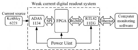
In this experimental system, the current source adopted the easy-to-use programmable current source Keithley 6221 whose range of output DC current is 100 fA ~ 100 mA with ultra-low current noise and the weak current measurement employed the ADAS1134 current-digital converter of Analog Devices. The internal integrator of the ADAS1134 chip will integrate the current for a specified time to obtain the accumulated charge of the current in a period of time. The block diagram of the experimental system is shown in Figure 2: the ADAS1134 was used to collect the nA-level current output by the Keithley 6221 current source; the FPGA obtained the digital quantity corresponding to the charge collected by the ADAS1134 through the SPI interface; then the FPGA converted the digital quantity into the current value which was sent to the PC acquisition software via Ethernet (RTL8211EG is the PHY chip); the PC acquisition software did acquire, display and store weak current data. The actual experiment system is shown in Figure 3.
Figure 2. The diagram experimental system
Figure 3. The device of weak current measurement system
3.2 Error correction process
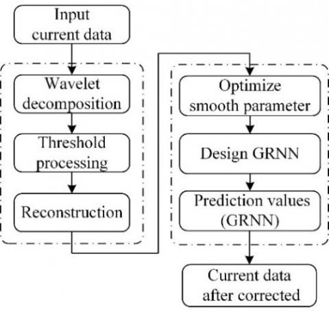
Figure 4 is a block diagram of the error correction process to measurement system proposed for the weak current in this paper. The system is mainly composed of wavelet denoising and GRNN model. Performed wavelet denoising pre-processing on the measured weak current data, and then used the GRNN model for error correction on the denoised weak current data. These two main parts are discussed detailedly in Section 4.
Figure 4. The block diagram of the proposed error correction system
In this work, the Keithley 6221 current source output current range was set to 1-700 nA, and the current output step value was 0.1 nA. The weak current digital readout system and PC acquisition software in the experimental system were used to continuously collect each point of current output by Keithley 6221 current source. The current of each point was continuously collected 200 times, and 1,400,000 weak current measurement data samples were obtained in total. These samples were used as the weak current data set of this experiment to verify the performance of the method followed in Section 2 of this paper. In order to meet the performance requirements of the simulation system for the simulation experiment, a computing system (64 bit 32 GB RAM, 3.6 GHz) is used for current measurement error correction applications in MATLAB Version 2016.
4.1 Denoising
In order to denoise the collected weak current signal and obtain a better denoising effect, it is necessary to select an appropriate wavelet basis function and wavelet decomposition scale N. For the sake of evaluating the effect of wavelet denoising algorithm, the following indicators were used as evaluation criteria:
(1) Signal Noise Ratio (SNR), the formula is defined as follows:
$SNR=10\log [\frac{\sum\limits_{i=1}^{n}{f(i)}}{\sum\limits_{i=1}^{n}{{{(\hat{f}(i)-f(i))}^{2}}}}]$ (5)
(2) Root Mean Square Error (RMSE), its formula is defined as:
$RMSE=\sqrt{\frac{1}{\text{n}}{{\sum\limits_{i=1}^{n}{[\hat{f}(i)-f(i)]}}^{2}}}$ (6)
where, f(i) is the original signal, $\hat{f}(i)$ is the signal after wavelet denoising, and n is the number of sampling points. After the signal was denoised by wavelet, the value of SNR became larger and the value of RMSE got smaller, indicating that it is closer to the original signal, which can prove that the wavelet basis function and decomposition levels have better denoising effect. Haar and Daubechies (dbN) as wavelet bases were commonly used. This paper used Haar, db2, db3, db4, db5, db6 wavelet basis functions and different decomposition levels to denoise the collected weak current data. The corresponding denoising results are shown in Table 1.
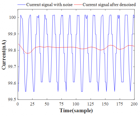
According to the experimental results in Table 1, db5 wavelet was used to decompose the weak current sampling data into four levels to realize denoising. The thresholds corresponding to the four levels are $\lambda_{\text {level } 1}=0.12, \lambda_{\text {level } 2}=0.22 , \lambda_{\text {level3 }}=2.00 \quad and \quad\lambda_{\text {level } 4}=1.49$ respectively. The SNR after denoised can reach 51.2041 which is higher than that of Haar wavelet and other Daubechies wavelets denoising. The RMSE after denoised is 1.1064, which is smaller than that of Haar wavelet and other Daubechies wavelets denoising. Therefore, this paper used db5 wavelet basis function to decompose the original weak current sampling data in four levels. Figure 5 shows the denoised result of the actual measurement of weak current data in the experimental system when Keithley 6221 output a standard current of 100 nA.
Table 1. The denoised effect of different wavelet bases and decomposition levels (the DL is decomposition level)
|
Wavelet |
DL |
SNR |
RMSE |
Wavelet |
DL |
SNR |
RMSE |
|
Haar |
1 |
50.8282 |
1.1664 |
db4 |
1 |
50.8542 |
1.1629 |
|
2 |
50.8640 |
1.1616 |
2 |
50.8755 |
1.1600 |
||
|
3 |
50.9160 |
1.1546 |
3 |
50.9556 |
1.1494 |
||
|
4 |
50.9387 |
1.1516 |
4 |
50.9783 |
1.1464 |
||
|
db2 |
1 |
50.8540 |
1.1629 |
db5 |
1 |
50.8560 |
1.1626 |
|
2 |
50.8802 |
1.1594 |
2 |
50.8761 |
1.1600 |
||
|
3 |
50.9488 |
1.1503 |
3 |
50.9799 |
1.1462 |
||
|
4 |
50.9755 |
1.1468 |
4 |
51.2041 |
1.1064 |
||
|
db3 |
1 |
50.8525 |
1.1631 |
db6 |
1 |
50.8559 |
1.1627 |
|
2 |
50.8749 |
1.1601 |
2 |
50.8745 |
1.1602 |
||
|
3 |
50.9514 |
1.1499 |
3 |
50.9617 |
1.1486 |
||
|
4 |
50.9764 |
1.1466 |
4 |
50.9803 |
1.1461 |
Figure 5. The effect of Wavelet threshold denoising
The blue curve in Figure 5 is the actual sampling data curve of the weak current, and the red curve is the weak current signal curve through wavelet denoising. It can be seen from Figure 5 that the db5 wavelet base is used to decompose the weak current signal into four levels to achieve the denoising effect, which can achieve the purpose of data preprocessing.
4.2 Current measurement error correction based on GRNN model
In this paper, the actual sample data of weak current signals were denoised as the input of GRNN training and testing. Besides, the current value output by Keithley 6221 was taken as the output value of GRNN training and the expected value of test output. It can be seen from Figure 5 that 20 current value samples can be obtained by continuously measuring the current value output from Keithley 6221, and the complete and effective sampling of one current value can be finished. Therefore, 20 consecutive samples were randomly selected from every 200 continuous current data samples in the dataset to obtain 140,000 current data samples, which constituted the dataset of GRNN model training and testing in this experiment. In the new data set, 70% of the 20 samples measured for each current value of Keithley 6221 output were used for the construction of GRNN model, and the remaining 30% of the data samples were used to test the performance of the constructed GRNN model.
In order to evaluate the performance of the proposed algorithm model, the mean square error (MSE), root mean square error (RMSE), mean absolute error (MAE) and mean absolute percentage error (MAPE) were used as evaluation criteria, and the corresponding formula was Eq. (7)-(10).
(1) Mean Square Error(MSE):
$MSE=\frac{1}{\text{n}}{{\sum\limits_{i=1}^{n}{[{{x}_{i}}-{{{\hat{x}}}_{i}}]}}^{2}}$ (7)
(2) Root Mean Square Error(RMSE):
$RMSE=\sqrt{\frac{1}{\text{n}}{{\sum\limits_{i=1}^{n}{[{{x}_{i}}-{{{\hat{x}}}_{i}}]}}^{2}}}$ (8)
(3) Mean Absolute Error(MAE):
$MAE=\frac{1}{\text{n}}\sum\limits_{i=1}^{n}{\left| {{x}_{i}}-{{{\hat{x}}}_{i}} \right|}$ (9)
(4) Mean Absolute Percentage Error(MAPE):
$MAPE=\frac{1}{\text{n}}\sum\limits_{i=1}^{n}{\left| \frac{{{x}_{i}}-{{{\hat{x}}}_{i}}}{{{x}_{i}}} \right|}\times 100%$ (10)
In the above formulas: xi is the actual value, $\hat{x}_i$ is the model predicted value, and n is the number of samples.
In GRNN model, σ is the only parameter that needs to be adjusted; too large σ will lead to the smoother output of GRNN model, and the consequent error will increase; too small σ will lead to overfitting for the output of GRNN model. Therefore, the choice of σ value will have a decisive impact on the performance of GRNN model. In this paper, the grid search method was used to optimize the smoothing parameter, and the K-fold cross validation was carried out for the GRNN model to avoid overfitting and under fitting. MSE was used as the criteria for the performance evaluation of cross validation. The $\left[\sigma_{\text {Low }}, \sigma_{\text {High }}\right]$ was divided into N equal parts, and the σ value was iteratively selected in $\left[\sigma_{\text {Low }}, \sigma_{\text {High }}\right]$. The definition of σ value is shown in Eq. (11).
$\sigma ={{\sigma }_{Low}}+(k-1)\frac{{{\sigma }_{High}}-{{\sigma }_{Low}}}{N}$ (11)
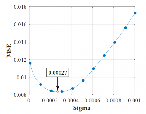
Figure 6. The cross-validation cure for GRNN model (Optimal σ=0. 00027)
The optimal σ value was selected according to the minimum average MSE. In this paper, the optimization range of σ value was set as [0.00001,0.001], and the iteration times ‘m’ was 100. Figure 6 shows the effect of the smoothing parameter σ on the GRNN model. The curve has an obvious minimum value, and that is, the best value of the smoothing parameter σ is 0.00027.
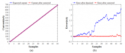
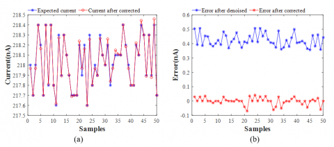
In order to verify the effectiveness of the error correction model proposed in current measurement, the GRNN model was constructed by using the optimal parameter and training set, the weak current measurement value in the test set was used as the input of the constructed GRNN model, and the current correction output value of the constructed GRNN model can be obtained. Take 50 samples from the test set at fixed intervals to test the GRNN model. The corresponding results of correction output are shown in Figure 7(a), and the measurement errors without and with correction are displayed in Figure 7(b). It can be seen from Figure 7(b) that the measurement error of the weak current in the experimental system increases with the increase of the measured current, but the corrected output error of the GRNN model is not affected (the error is close to 0). Forasmuch as the above analyzed results, the GRNN model proposed in this work is effective in correcting the measurement error of weak current.
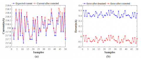
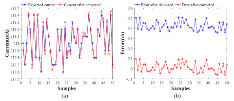
In this paper, the GRNN model was also compared with the least squares model and the BPNN model, and the performance of each model were evaluated via RMSE, MAE, and MAPE values. After least square fitting, BPNN model training and GRNN modelling were conducted through the same training dataset, 50 consecutive samples in the test set were randomly taken as the input of every correction model, and the corresponding correction output effect diagram and error comparison diagram are shown in Figures 8-10. Table 2 shows the corresponding correction output results of these several correction algorithms at different current measurement values. As can be seen from Figures 8-10 and Table 2, the error between the weak current value output by the least squares model and BPNN model correction and the standard value output by Keithley 6221 for weak current is smaller than the measurement error of the experimental system. However, the GRNN model obviously has a better correction effect on the measurement error of the experimental system.
The results of performance comparison for each correction method are clearly exhibited in Table 3 after taking the same training dataset to perform least squares fitting, BPNN model training, and GRNN model construction, respectively, and then taking the overall test set sample for weak current correction output. The standlone approach in Table 3 indicates that different correction models are fitted, trained and constructed by using the measured weak current data with noise as the dataset, and then the performances of corresponding models are tested. The wavelet denoising method in Table 3 shows that the same data as standlone approach were denoised and then were used as a dataset to fit, train and construct different correction models, separately. After that, the performances of corresponding models were tested. It can be seen from Table 3 that compared with preprocessing without wavelet threshold denoising, the use of wavelet threshold denoising to preprocess the original data improves the correction performance of each error correction model. Meanwhile, the weak current data sample was denoised by wavelet, and then the weak current measurement error was corrected by GRNN. The result corrected is that RMSE=0.0911 nA, MAE=0.0354 nA, MAPE=0.0078%. The RMSE value before corrected is 12.14 times as much as the RMSE value after corrected, and the RMSE value through the correction is smaller than that with the least square method and BPNN correction respectively. The experimental results show that the method of combining wavelet denoising and GRNN correction model shows better correction performances for the measurement error of the weak current measurement system than the least square method and BPNN model. Because the GRNN model has strong nonlinear mapping capabilities, high fault tolerance and robustness, the GRNN model has achieved very good results in the current measurement error correction of the system.
Figure 7. The correction current output values (a) and the errors (b) after denoised and corrected of GRNN
Figure 8. The corrected current values (a) and the errors (b) after corrected and denoised of least square (when the output current of Keithley 6221 is 217.6-218.4 nA)
Figure 9. The corrected current values (a) and the errors (b) after corrected and denoised of BPNN (when the output current of Keithley 6221 is 217.6-218.4 nA)
Figure 10. The corrected current values (a) and the errors (b) after corrected and denoised of GRNN (when the output current of Keithley 6221 is 217.6-218.4 nA)
Table 2. The corrected output results of different algorithms (nA)
|
Keithley 6221 |
Measure |
Least-square |
BPNN |
GRNN |
||||
|
Value |
Error |
Correction value |
Error |
Correction value |
Error |
Correction value |
Error |
|
|
43.5 |
43.4473 |
0.0527 |
43.4430 |
0.0570 |
43.4860 |
0.0140 |
43.4994 |
0.0006 |
|
73.4 |
73.2723 |
0.1277 |
73.3116 |
0.0884 |
73.3599 |
0.0401 |
73.3959 |
0.0041 |
|
140 |
139.6953 |
0.3047 |
139.8980 |
0.1020 |
139.9139 |
0.0861 |
139.9956 |
0.0044 |
|
180.5 |
180.2135 |
0.2865 |
180.5531 |
-0.0531 |
180.4526 |
0.0474 |
180.4954 |
0.0046 |
|
228.5 |
228.0392 |
0.4608 |
228.5676 |
-0.0676 |
228.4990 |
0.0010 |
228.5004 |
-0.0004 |
|
252.4 |
252.2220 |
0.1780 |
252.8546 |
-0.4546 |
252.5619 |
-0.1619 |
252.3607 |
0.0393 |
|
300.7 |
299.8450 |
0.8550 |
300.6942 |
0.0058 |
300.4764 |
0.2236 |
300.6988 |
0.0012 |
|
379.7 |
378.1932 |
1.5068 |
379.4114 |
0.2886 |
379.6262 |
0.0738 |
379.6994 |
0.0006 |
|
403.7 |
402.0798 |
1.6202 |
403.4087 |
0.2913 |
403.7229 |
-0.0229 |
403.6924 |
0.0076 |
|
448.2 |
446.3686 |
1.8314 |
447.8945 |
0.3055 |
448.2430 |
-0.0430 |
448.1955 |
0.0045 |
|
534.2 |
532.3661 |
1.8339 |
534.2208 |
-0.0208 |
533.9456 |
0.2544 |
534.0451 |
0.1549 |
|
575.2 |
573.3181 |
1.8819 |
575.2924 |
-0.0924 |
575.1292 |
0.0708 |
575.1388 |
0.0612 |
|
625.7 |
623.3911 |
2.3089 |
625.4681 |
0.2319 |
625.3898 |
0.3102 |
625.6933 |
0.0067 |
|
699.8 |
697.1903 |
2.6097 |
699.3113 |
0.4887 |
699.7591 |
0.0409 |
699.7814 |
0.0186 |
Table 3. The corrected output performances of different models
|
|
Standlone approach |
Wavelet denoising approach |
||||
|
Criteria |
RMSE (nA) |
MAE (nA) |
MAPE (%) |
RMSE (nA) |
MAE (nA) |
MAPE (%) |
|
Before correction |
1.3523 |
1.0883 |
0.34 |
1.1064 |
0.9456 |
0.22 |
|
Least-square |
0.3313 |
0.2556 |
0.16 |
0.2523 |
0.1882 |
0.0681 |
|
BPNN |
0.2639 |
0.2029 |
0.14 |
0.1517 |
0.0968 |
0.0380 |
|
GRNN |
0.2405 |
0.1887 |
0.14 |
0.0911 |
0.0354 |
0.0078 |
This work proposed a measurement error correction technique for the weak current measurement system based on the combination of wavelet denoising and GRNN model to reduce the measurement error of the weak current measurement system caused by some factors such as noise and leakage current at input. Wavelet denoising was applied to the weak current data collected by the experimental system to improve the correction ability of GRNN model. Finally, GRNN was used to correct the weak current sample data by means of wavelet denoising and compared with the correction method based on least square method and BPNN. The experimental results showed that the preprocessing of data by wavelet denoising can better improve the correction performance of every error correction model. In addition, the correction effect of wavelet denoising combined with GRNN was better than that of wavelet denoising combined with least square method and BPNN respectively, and RMSE = 0.0911 nA, MAE = 0.0354 nA, MAPE = 0.0078%, which were greatly improved by combining wavelet denoising with GRNN. Consequently, the error correction method of wavelet denoising combined with GRNN proposed in this paper owns a good correction effect on the measurement error of the weak current measurement system. In addition, in terms of software algorithm, a reference method has been proposed, which is useful, practical and significant.
This research is supported by the Special Fund Project for Guiding Scientific and Technological Innovation of Gansu Province, China (Grant No. 2019zx-10).
[1] Hu, H.Q., Gao, Q.F., Shen, S.S. (2016). Design of a high precision and wide range weak current detection preamplifier circuit. Nuclear Electronics & Detection Technology, 36(8): 847-851. https://doi.org/10.3969/j.issn.0258-0934.2016.08.017
[2] Lei, S.J., Wei, Z.Y., Chen, G.Y., Zhang, Z.X., Huang, S.B., Fang, M.H. (2010). Design of weak current measurement circuit in space particle detector. Journal of Astronautic Metrology & Measurement, 30(6): 45-50. https://doi.org/10.3969/j.issn.1000-7202.2010.06.010
[3] Tan, X., Chen, S., Yan, X., Fan, Y., Min, H., Wang, J. (2016). A highly sensitive wide-range weak current detection circuit for implantable glucose monitoring. IEICE Electronics Express, 13(8): 20150616-20150616. https://doi.org/10.1587/elex.13.20150616
[4] Li, J.L., Chen, T., Li, K. (2018). Research on capacitor leakage current measurement technique. Industrial Control Computer, 31(4): 144-146. https://doi.org/10.3969/j.issn.1001-182X.2018.04.062
[5] Xu, Z., Mao, R., Duan, L., She, Q., Hu, Z., Li, H., Lu, Z., Zhao, Q., Yang, H., Su, H. (2013). A new multi-strip ionization chamber used as online beam monitor for heavy ion therapy. Nuclear Instruments and Methods in Physics Research Section A: Accelerators, Spectrometers, Detectors and Associated Equipment, 729: 895-899. https://doi.org/10.1016/j.nima.2013.08.069
[6] Wang, J., Li, B.K., Ruan, L.B., Tian, G., Li, X.B., Qu, H.G. (2012). Automatic weak-current measurement system with high precision. High Power Laser & Particle Beams, 24(08): 1975-1979. https://doi.org/10.3788/HPLPB20122408.1975
[7] Guo, Z., Liu, G., Wu, S., Mao, L. (2017). Research on design of weak current measurement system based on I-V convertor. International Conference on Materials Science. https://doi.org/10.2991/msmee-17.2017.159
[8] Shenoy, V., Jung, S., Yoon, Y., Park, Y., Kim, H., Chung, H.J. (2014). A CMOS analog correlator-based painless nonenzymatic glucose sensor readout circuit. IEEE Sensors Journal, 14(5): 1591-1599. https://doi.org/10.1109/JSEN.2014.2300475
[9] Kim, D., Goldstein, B., Tang, W., Sigworth, F.J., Culurciello, E. (2012). Noise analysis and performance comparison of low current measurement systems for biomedical applications. IEEE Transactions on Biomedical Circuits and Systems, 7(1): 52-62. https://doi.org/10.1109/TBCAS.2012.2192273
[10] Zhang, G.Y., Tuo, X.G., Wang, H.H., Xi, D.S., Zhang, Z.Y. (2011). Comparison and improvement with the capacity of C/R measurement method of fA level current. Electrical Measurement & Instrumentation, 48(552): 8-12. https://doi.org/10.3969/j.issn.1001-1390.2011.12.003
[11] Wang, W., Cui, M., Li, M.W, Zhang, P., Wu, Q.N., Zhang, S.N. (2019). Design of pA level current signal detection circuit. Journal of North University of China (Natural Science Edition), 40(2): 173-179. https://doi.org/10.3969/j.issn.1673-3193.2019.02.014
[12] Hao, S.L., Tuo, X.G., Wang, H.H., Xi, D.S. (2012). Design of ionization chamber current measuring instrument based on DDC112. Nuclear Electronics & Detection Technology, 32(11): 1309-1313, 1335. https://doi.org/10.3969/j.issn.0258-0934.2012.11.019
[13] Campisi-Pinto, S., Adamowski, J., Oron, G. (2012). Forecasting urban water demand via wavelet-denoising and neural network models. Case study: City of Syracuse, Italy. Water Resources Management, 26(12): 3539-3558. https://doi.org/10.1007/s11269-012-0089-y
[14] Cui, Z., Wang, Y.X. (2019). Denoising of seismic signals through wavelet transform based on entropy and inter-scale correlation model. Instrumentation Mesure Métrologie, 18(3): 289-295. https://doi.org/10.18280/i2m.180309
[15] Chen, J., Li, X., Mohamed, M.A., Jin, T. (2020). An adaptive matrix pencil algorithm based-wavelet soft-threshold denoising for analysis of low frequency oscillation in power systems. IEEE Access, 8: 7244-7255. https://doi.org/10.1109/ACCESS.2020.2963953
[16] Srivastava, M., Anderson, C.L., Freed, J.H. (2016). A new wavelet denoising method for selecting decomposition levels and noise thresholds. IEEE Access, 4: 3862-3877. https://doi.org/10.1109/ACCESS.2016.2587581
[17] Cheng, H., Yuan, Y., Wang, E.D., Fu, J.F. (2018). Study of hierarchical adaptive threshold micro-seismic signal denoising based on wavelet transform. Journal of Northeastern University (Natural Science), 39(9): 1332-1336. https://doi.org/10.12068/j.issn.1005-3026.2018.09.023
[18] Schimmack, M., Mercorelli, P. (2018). An on-line orthogonal wavelet denoising algorithm for high-resolution surface scans. Journal of the Franklin Institute, 355(18): 9245-9270. https://doi.org/10.1016/j.jfranklin.2017.05.042
[19] Bendu, H., Deepak, B.B.V.L., Murugan, S. (2017). Multi-objective optimization of ethanol fuelled HCCI engine performance using hybrid GRNN–PSO. Applied Energy, 187: 601-611. https://doi.org/10.1016/j.apenergy.2016.11.072
[20] Bendu, H., Deepak, B., Murugan, S. (2016). Application of GRNN for the prediction of performance and exhaust emissions in HCCI engine using ethanol. Energy Conversion and Management, 122: 165-173. https://doi.org/10.1016/j.enconman.2016.05.061
[21] Li, W.D., Yang, X., Li, H., Su, L.L. (2017). Hybrid forecasting approach based on GRNN neural network and SVR machine for electricity demand forecasting. Energies, 10(1): 44. https://doi.org/10.3390/en10010044