Fethi Albouchi* | Jemni Abdelmajid
© 2021 IIETA. This article is published by IIETA and is licensed under the CC BY 4.0 license (http://creativecommons.org/licenses/by/4.0/).
OPEN ACCESS
The present experimental paper investigated the measurement of the conductive and the optical parameters of liquids using a photothermal technique related to an inverse problem. The method consists in heating with a halogen lamp, the front face of a cell containing the liquid sample, and measuring the heating and the cooling process of the rear face using an open junction thermocouple. The numerical model is developed by the thermal quadrupole method taking into account conduction and radiation heat transfer in the liquid.
Measurements performed on several liquids validate the method. Good agreement is found between the obtained values of the thermal properties and previously reported values in literature. Moreover, measurements under the photothermal technique are less time consuming than using the classical electrothermal method. Due to its noncontact nature, this method may find practical application for the thermal characterization of complex fluids essentially nanofluids.
liquids, optical parameters, parameter estimation, photothermal method
In recent years, nanofluid technology occupies the foremost area in engineering field. Their potential applications are numerous and very important in several fields: electronic cooling, aeronautics and space. These Nanofluids are colloidal solutions consisting of particles of nanometric size suspended in a base fluid. The basic liquids generally used in the preparation of nanofluids are those frequently used in thermal applications such as water, ethylene glycol and motor oil. In many industrial applications, the percentage of the base fluid is more than 95%. For a good manufacturing of lubricants, it was necessary to know the properties of basic fluids, essentially the thermal conductivity [1, 2].
Different methods are developed for measuring the thermal properties of liquid. Two types of methods are generally used (electrothermal and photothermal methods). The one most used for measuring the liquid thermal conductivity is the hot wire method. This technique is based on an analytical technique. The disadvantage of this method is the low precision due to the choice of the linear interval on the experimental signal [3-10].
Some works deal with photothermal characterization of liquids [11-18]. The Flash method which is principally developed for characterization of solids is adapted by Coquard and Panel [15] for measuring the thermal conductivity of liquids. In their work they use a sample in the form of three layers constituting a cell containing the liquid. This cell is then assumed to a one layer. Remy and Degiovanni [16, 17] show that the presence of several thermal transfer modes presents a difficulty for the measurement of the thermal properties of liquids.
The objective of this paper is to implement an experimental technique associated to an inverse problem to measure liquids thermal and optical parameters. In this technique the liquid is placed in a Teflon cell closed by two solid strips. The sample is excited on its front face by a crenel heat flux and the temperature response is measured on the rear face. In this study, we investigate the interest of a conductive-radiative heat transfer model and the simultaneous estimation of the conductive and optical properties.
For this reason, a thermal model is developed to predict heat transfer within liquids. This model, taking into account the conductive and radiative heat transfers, is built with the quadrupole technique [19]. Using the inverse procedure, the identification of the thermophysical properties is based on the minimization of the difference between measurements and the calculated temperatures. The obtained results are presented and validated with literature values.
2.1 Spectroscopic measurement of the normal transmittance
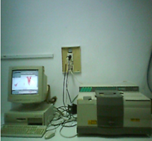
Three processes (transmission, absorption, and reflection) can occur if an incident flow falls on a medium or a surface. In this study, the normal transmittance measurements are performed by a Nicolet-560 FTIR spectrometer (Figure 1). During measurements, a background spectrum was recorded while the compartment was empty before each sample was scanned. The samples are placed in the normal direction between the source and the detector. Then, several measurements were conducted for each sample and a mean value is then calculated.
Figure 1. Experimental setup for transmittance measurements
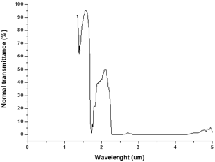
Figure 2. Normal transmittance for oil
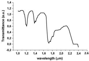
Figure 3. Transmittance for paraffin oil [20]
Two samples water and oil are used in this study. The obtained curve for oil sample is illustrated on Figure 2. We remark that the normal transmittance presents maxima in the wave length range of [$1.2 \mu \mathrm{m}-2.3 \mu \mathrm{m}$]. The spectrum shows that the maxima are located in the range of $1.3 \mu \mathrm{m}-2.2 \mu \mathrm{m}$. This figure shows that strong absorption bands exist for oil at 1200–1350 nm and again at 1680 -1750 nm. In addition at nearly 1480 nm, 2000 nm and 2100 nm this fluid is essentially opaque to incoming radiation.
Figure 3 illustrates FTNIR transmittance of paraffin oil measured by Saadallah et al. [20]. The comparison between the curves (2) and (3) shows that our results are in good agreement over a majority of the spectral wave length range with those found by Faycel Saadallah [20].
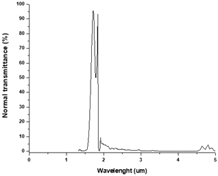
On Figure 4, we present the normal transmittance for water sample. It can be seen that the maxima are located in the range of $1.6 \mu \mathrm{m}-2 \mu \mathrm{m}$. We note three strong absorption maxima at 1650, 1750 nm and at 1850 nm. Furthermore, water is opaque at nearly 1600 nm, 1800 nm and 1950 nm These results are in agreement with the values given by Ai et al. [21].
Figure 4. Normal transmittance for water
2.2 Measurement of absorption coefficient
To confirm the values obtained by the inverse method, we measure the optical thickness coefficient using the spectroscopic transmittance technique. In this case, we perform normal transmittance measurements [22].
We use the theory of reflectivity and transmittance in the case of a normal incidence to calculate the radiative absorption coefficients. The reflectance R (at the window-liquid interface) can be calculated using the Fresnel’s relations [21]:
$r={{\left( \frac{{{n}_{r}}-1}{{{n}_{r}}+1} \right)}^{2}}$ (1)
The transmittance is then given by [23]:
${{T}_{r}}=\frac{{{I}_{t}}}{{{I}_{0}}}=\frac{{{(1-r)}^{2}}\exp (-{{k}_{a}}e)}{1-{{r}^{2}}\exp (-2{{k}_{a}}e)}$ (2)
With ka is the absorption coefficient of liquid with e thickness. Using this formulation, a mean value of the absorption coefficient is calculated from Eq. (2) and the obtained results are tabulated in Table 1.
Table 1. Comparison between inverse and direct measurement for radiative absorption
|
Sample |
Arithmetic mean values (normal transmittance measurements) |
Relative uncertainty (%) |
|
Water |
316.64 m-1 |
2.83 |
|
Oil |
832.31 m-1 |
3.32 |
The measurement of these two parameters is performed using an inverse estimation based on the calculation of the gap between the theoretical and the experimental temperatures. The theoretical temperatures are the output of a thermal model developed by the quadrupole formalism. This theoretical model describes the heat transfer by conduction and radiation. The sample is heated on its front face and the response is measured on the rear face of the sample.
3.1 Experimental device
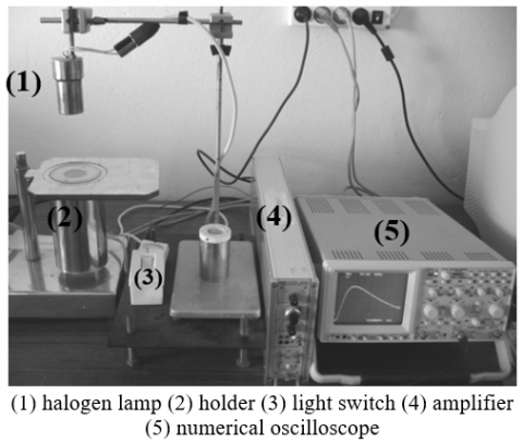
The Figure 5 presents the experimental device. A halogen lamp of power 1200 Wm-2 ensures the flow of excitation on the front face. The sample is placed in the enclosure on an open junction thermocouple of sensitivity 360 μV/K. An amplifier is used to amplify the thermocouple signal and saved on a numerical oscilloscope (HAMEG HM-407). Then, the measured signal is transferred to a computer using the RS 232 interface serial and the SP 107 software.
Figure 5. Experimental apparatus
3.2 Theoretical model
The physical model illustrated in Figure 6 describes conductive and radiative heat transfer in the sample. In this case, the different layers are supposed to be plane parallel, grey and isotropic semi-transparent medium. For boundary conditions, we consider that the lateral heat loss is neglected and the heat transfer on the two faces with the surrounding environment is expressed by heat transfer coefficient h. In fact, based on precedent works [24, 25] and for small temperature rise within the sample, we can neglect the convective effects in the liquid.
In this case, a finite pulse heat flux (Eq. (3)) is submitted to the front face of the sample at t=0.
$Q=\left\{ \begin{align} & \psi \,\,\,\,\,0\le t\le {{t}_{c}} \\ & 0\,\,\,\,\,\,\,\,t\ge {{t}_{c}} \\\end{align} \right\}$ (3)
where, tc is the duration of the applied heating. The sample is initially assumed at uniform temperature T0.
Figure 6. Physical model
The energy equation describing heat transfer in the sample is expressed as:
$-\frac{\partial }{\partial z}\left( -\lambda \frac{\partial T(z,t)}{\partial z}+{{q}_{r}} \right)=\rho \,{{c}_{p}}\frac{\partial T}{\partial t}$ (4)
In this regard, for solving the system of equation, we assume the following parameters presented in the Table 2.
Table 2. Parameters used in the thermal model
|
Dimensionless temperature |
$\theta=T^{*}-T_{0}^{*}=\frac{T-T_{0}}{\left(\psi / \rho c_{p} e\right)}$ |
|
Dimensionless time |
$t^{*}=\frac{a t}{e^{2}}$ |
|
Dimensionless space variable |
$z^{*}=\frac{Z}{e}$ |
|
Optical thickness |
$\tau_{0}=\left(k_{a}+k_{d}\right) \cdot e$ |
|
Planck number |
$N_{p l}=\frac{\lambda k_{a}}{4 n_{r}^{2} \bar{\sigma} T_{0}^{3}}$ |
|
Dimensionless radiative flux |
$q_{r}^{*}=\frac{q_{r}}{4 n_{r}^{2} \bar{\sigma} T_{0}^{4}}$ |
|
Dimensionless intensities |
$I^{*}=\frac{\pi I}{4 n_{r}^{2} \bar{\sigma} T_{0}^{4}}$ |
Using these dimensionless variables, we can write the Eq. (4) in the following form:
$\frac{\partial \theta }{\partial {{t}^{*}}}=\frac{{{\partial }^{2}}\theta }{\partial {{z}^{*}}^{2}}-\frac{{{\tau }_{0}}{{T}_{0}}}{{{N}_{pl}}}\frac{\partial q_{r}^{{}}}{\partial {{z}^{*}}}$ 0<z*<1 (5)
Using the approximation of azimuthally symmetric radiation, the radiative transfer equation in the semi-transparent medium can be written as:
$\frac{\partial I(s,\Delta )}{\partial s}+{{\beta }_{e}}I(s,\Delta )=S\,$ (6)
where, $S=k_{a} I_{b}+\frac{k_{d}}{4 \pi} \int_{4 \pi} P\left(\mu, \mu^{\prime}\right) I(z, \mu) d \mu^{\prime}$
The extinction coefficient is given by $\beta_{e}=k_{a}+k_{d}$, $I_{b}$ is the intensity of the black body and $\mu=\cos (\gamma)$ is the cosine of the direction vector.
The radiative flux vector is calculated by the integral of the intensity over the spherical space:
${{\vec{q}}_{r}}(s)=\int_{4\pi }{\vec{I}(s,\vec{\Delta })\vec{\Delta }d\Omega }$ (7)
Using the radiative intensity, the radiative flux can be written as:
${{q}_{r}}\left( z \right)={{I}^{+}}-{{I}^{-}}$ (8)
In the front face, the radiative boundary condition for opaque, diffusely emitting, diffusely reflecting interface is given by [26]:
$\begin{align} & {{I}^{+}}(0)={{\varepsilon }_{1}}{{I}^{0}}({{T}_{1}})+{{r}_{1}}\frac{\int_{0}^{2\pi }{\int_{-1}^{0}{{{I}^{-}}(0,\mu ')\mu 'd\mu 'd\Phi '\,}}}{\int_{0}^{2\pi }{\int_{-1}^{0}{\mu 'd\mu 'd\Phi '\,}}} \\ & \,\,\,\,\,\,\,\,\,\,\,\,\,={{\varepsilon }_{1}}{{I}^{0}}({{T}_{1}})+2{{r}_{1}}\int_{0}^{1}{{{I}^{-}}(0,-\mu ')\mu 'd\mu '\,\,\,\,\,\,} \\\end{align}$ (9)
Similarly, in the rear face (z=1), this condition is written as:
$\begin{align} & {{I}^{+}}(1)={{\varepsilon }_{2}}{{I}^{0}}({{T}_{2}})+{{r}_{2}}\frac{\int_{0}^{2\pi }{\int_{-1}^{0}{{{I}^{-}}(0,\mu ')\mu 'd\mu 'd\Phi '\,}}}{\int_{0}^{2\pi }{\int_{-1}^{0}{\mu 'd\mu 'd\Phi '\,}}} \\ & \,\,\,\,\,\,\,\,\,\,\,\,\,={{\varepsilon }_{2}}{{I}^{0}}({{T}_{2}})+2{{r}_{2}}\int_{0}^{1}{{{I}^{-}}(0,\mu ')\mu 'd\mu '\,\,\,\,\,\,\,} \\\end{align}$ (10)
In absorbing emitting medium, one can write the reduced radiative flux as:
$\begin{align} & {{q}_{r}}(z)={{I}^{+}}(0){{e}^{-{{\tau }_{0}}z}}-{{I}^{-}}(1){{e}^{-{{\tau }_{0}}(1-z)}} \\ & -\frac{1}{4}({{e}^{-{{\tau }_{0}}z}}-{{e}^{-{{\tau }_{0}}(1-z)}}) \\ & +\frac{{{\tau }_{0}}}{{{T}_{0}}}\int_{0}^{z}{\theta (z')\exp (-{{\tau }_{0}}(z-z'))dz'-} \\ & \frac{{{\tau }_{0}}}{{{T}_{0}}}\int_{z}^{1}{\theta (z')\exp (-{{\tau }_{0}}(z-z'))dz'} \\\end{align}$ (11)
Here I+(0), I-(1) are the dimensionless intensities given by the radiative boundary conditions.
The entire sample is assumed to be one layer of thickness e. In this case, in the Laplace space, the Eq. (4) can be written as:
$\frac{{{d}^{4}}\bar{\theta }}{d{{z}^{*}}^{4}}-\left( p+2\frac{{{\tau }^{2}}}{N}+{{\tau }^{2}} \right)\frac{{{d}^{2}}\bar{\theta }}{d{{z}^{*}}^{2}}+p{{\tau }^{2}}\bar{\theta }=0$ (12)
with $N=(3 / 2) N_{p l}$.
The thermal quadrupole formulation [19] is used to solve equation (12). The system is then represented by:
$\left(\begin{array}{l}\bar{\theta}(0) \\ \bar{\phi}(0)\end{array}\right)=\left(\begin{array}{ll}1 & 0 \\ B i & 1\end{array}\right)\left(\begin{array}{ll}A & B \\ C & D\end{array}\right)\left(\begin{array}{ll}1 & 0 \\ B i & 1\end{array}\right)\left(\begin{array}{c}\bar{\theta}(1) \\ 0\end{array}\right)$ (13)
where, Bi is the Biot number defined as $B i=\frac{h . e}{\lambda}$
The temperature of the rear face can be calculated by solving the system of equations in the space of the Laplace:
$\bar{\theta }\left( 1 \right)=\frac{\bar{\phi }\left( 0 \right)}{Bi\left( A+D+B.Bi \right)+C}$ (14)
where, $\bar{\phi}(0)=\frac{\xi_{c}}{p}\left[1-\exp \left(-t_{c} p\right)\right]$ is the crenel excitation in the Laplace space.
We use the inverse Laplace transform to calculate the temperature T(t) [19].
3.3 Parameter estimation
3.3.1 Parameter estimation method
Numerous algorithms are used to solve the inverse heat problems. In the present study, we use the ordinary least squares (OLS) formulation [27]. This criterion is given by:
$\Gamma(p)=\sum_{i=1}^{n}\left(T_{m, i}-T_{c, i}(p)\right)^{2}$ (15)
In Eq. (15), the vector β presents the unknown parameters, Tm and Tc are respectively the measured and the calculated temperatures, and n is the number of measurements.
The minimization process is based on the Gauss-Newton algorithm and the solution vector is written as:
$p_{k+1}=p_{k}+\left[X\left(p_{k}\right)^{t} X\left(p_{k}\right)\right]^{-1} X\left(p_{k}\right)^{t}\left[T_{m}-T_{c}\left(p_{k}\right)\right]$ (16)
where, $p_{k+1}$ is the parameter vector on the iteration (k+1) and X is the sensitivity matrix defined in the next paragraph.
3.3.2 Analysis of the simultaneous parameter estimation
The sensitivity coefficients are beneficial to predict the estimation feasibility. Using the reduced form of these coefficients, we can write:
$Z_{i j}(t)=p_{j} X_{i j}\left(t_{i}, p\right)=p_{j} \frac{\partial T\left(t_{i}, p\right)}{\partial p_{j}}$ (17)
Using the reduced Hessian matrix $J=Z^{t} Z$ and the variance of the measurement noise $\sigma_{n}^{2}$, we can calculate the relative uncertainty on the estimated parameters given by the matrix R:
$R={{J}^{-1}}\sigma _{n}^{2}$ (18)
This uncertainty strongly depends on the noise level.
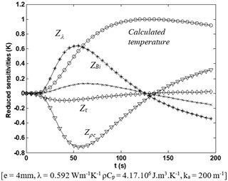
Figure 7. Reduced sensitivities for water
Figure 8. Reduced sensitivities for oil
To reduce the number of parameters, we normalize the temperatures by their maxima. Looking at the figures of the sensitivity coefficients (7, 8), one remark that the reduced sensitivities are great at time less than 100s. Given that the curves reach their maxima at different times, the parameters are uncorrelated and can be estimated simultaneously.
The visual analysis of the reduced sensitivity is supported by the variance-covariance calculation. The correspondent matrices which represent the correlation factors between the parameters βi and βj are written as:
$r_{i j}=\frac{\operatorname{Cov}\left(p i p_{j}\right)}{\sqrt{\operatorname{Var}\left(p_{i}\right) \operatorname{Var}\left(p_{j}\right)}}$ (19)
The estimated parameter vector is $p=\left[\lambda, B_{i}, \rho C, \tau\right]$. The simultaneous estimation of two parameters is easily performed and more accurate when the correlation factor is smaller than 0.9 [27]. Tables 3, 4 illustrate the calculated correlation factor for oil and water.
Table 3. Correlation matrix for oil sample
|
|
ri1 |
ri2 |
ri3 |
ri4 |
|
r1j |
1 |
-0.168 |
0.815 |
-0.037 |
|
r2j |
-0.168 |
1 |
-0.653 |
-0.493 |
|
r3j |
0.815 |
-0.653 |
1 |
0.417 |
|
r4j |
-0.037 |
-0.493 |
0.417 |
1 |
Table 4. Correlation matrix for water sample
|
|
ri1 |
ri2 |
ri3 |
ri4 |
|
r1j |
1 |
-0.157 |
0.970 |
0.065 |
|
r2j |
-0.157 |
1 |
-0.326 |
-0.257 |
|
r3j |
0.970 |
-0.326 |
1.000 |
0.217 |
|
r4j |
0.065 |
-0.257 |
0.217 |
1 |
For oil, it can be seen from Table 2, that all the correlation factor are small than 0.9. This indicates that the parameters are uncorrelated. So, it is possible to estimate all the parameters simultaneously. Whereas, for water, one can see that the correlation coefficient between the first and the third parameter is greater than 0.9 (Table 3). As consequence, the estimation accuracy on these parameters will be small.
Giving that, we work at low temperature, the sensitivity of the radiative parameter still less important than conductive ones. From the analysis of the correlation matrix, we can expect that the uncertainty on the estimation of the extinction coefficient will be more important than these of the conductive parameters especially for the water sample.
3.3.3 Results and discussion
In this study, the experimental measurements are accomplished on two samples which are water and oil. The front face of the sample is subjected to a flow for fifteen minutes and the acquisition time step is 0.25s. For the identification of the unknown parameters, we use the Gauss-Newton algorithm. Several measurements are made for each sample and an average value is then calculated. Tables 5 and 6 present the obtained results at 300 K.
Table 5. Results of estimation for the oil sample
|
|
Estimated values |
Rel ative uncertainty |
Kuntner [28] |
Remy [12] |
|
τ |
4.61 |
3.13 % |
- |
- |
|
λ (Wm-1K-1) |
0.134 |
2.02 % |
0.14 |
0.13 |
|
Bi |
0.77 |
1.26 % |
- |
- |
|
ρc (Wm-3K-1) |
1.789 106 |
0.74 % |
1.74 106 |
1.8 106 |
Table 6. Results of estimation for the water sample
|
|
Estimated values |
Relative uncertainty |
Kuntner [28] |
Remy [12] |
|
τ |
2.31 |
7.46 % |
- |
- |
|
λ (Wm-1K-1) |
0.599 |
1.52 % |
0.598 |
0.621 |
|
Bi |
0.28 |
1.40 % |
- |
- |
|
ρc (Wm-3K-1) |
4.19 106 |
1.22 % |
4.17 106 |
4.38 106 |
Locking at the relative uncertainty values, we remark that all the parameters are estimated with good precision. The uncertainty of the conductive parameters does not exceed 2.02% for the two samples.
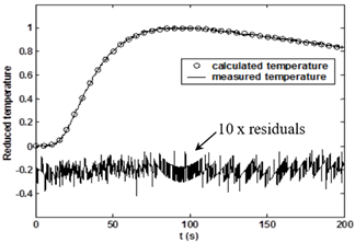
Figure 9. Measured and calculated temperatures and 10 x residuals for water sample
Despite the low reference temperature, the radiative parameter is well estimated in the case of the oil sample and the relative uncertainty is 3.13%. In the case of water, the relative uncertainty of the optical thickness (7.46%) is higher than this for oil (3.13%).
By comparison with bibliographic values, we remark that the estimated thermal conductivity values are very close to those given by Kuntner and Remy.
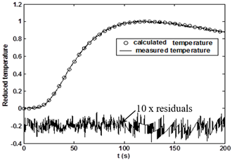
To validate the obtained results, we compared the calculated temperature and experimental measurements on Figure 9, 10. We note that the curves are very close. Locking at residuals curves (Figures 9, 10), we note a good agreement between the calculated and the experimental temperatures. The residuals are focused on zero and don’t present any fluctuations or aberrations.
Figure 10. Measured and calculated temperatures and 10 x residuals for oil sample
In Table 7, we present a comparison between the values of the absorption coefficient obtained by inverse estimation and direct measurement. We remark that the two methods give close values.
Table 7. Comparison between estimated and measured absorption coefficient
|
Sample |
Estimated values (inverse method) |
Arithmetic mean values (normal transmittance measurements) |
|
Water |
385 m-1 |
316.64 m-1 |
|
Oil |
768 m-1 |
832.31 m-1 |
In this work, we show that the rear-face photothermal method provides noncontact, fast, simultaneous and accurate measurements of the thermal conductivity and absorption coefficient of liquids. The estimated thermal conductivity is in good agreement with literature values, approving the applicability of the proposed method. We have shown that the thermal model is more sensitive to both the thermal conductivity and specific capacity than to optic thicknesses. Therefore, the estimation relative errors are large for optical parameters than for thermal parameters. In summary, it has been shown that our methodology, based on photothermal method associated to an inverse identification, can provide a complete thermal characterization of most common liquids used in science and technology.
Due to its noncontact nature, this method may find practical application for the thermal characterization of complex fluids essentially nanofluids.
This work is carried out in the Laboratory of Thermal and Energy Systems Studies. The authors wish to thank the mechanical unit for manufacturing the sample cell.
|
Ai, Bi, Ci, Di |
Matrix transfer coefficients of model i |
|
a |
Thermal diffusivity. (m2.s-1) |
|
Bi |
Biot number |
|
Γ |
OLS Norm |
|
cp |
Heat capacity (J.kg-1.K-1) |
|
e |
Sample thickness. (m) |
|
h |
Heat transfer coefficient. (W.m-2.K-1) |
|
I |
Radiative intensity. (W.m-2.str-1) |
|
J |
Hessian matrix |
|
k |
Absorption coefficient...(m-1) |
|
nr |
Refractive index |
|
Npl |
Planck number |
|
p |
Laplace parmeter |
|
qr |
Radiative heat flux...(W.m-2) |
|
Q |
Crenel excitation. (W.m-2) |
|
Rc |
Thermal contact resistance......(W-1.m2.K) |
|
r |
Surface reflectivity |
|
S |
Sample surface.(m2) |
|
t |
Time..(s) |
|
T |
Temperature..(K) |
|
T0 |
Reference temperature..(K) |
|
tc |
Heating time.(s) |
|
Tc |
Calculated temperature..(K) |
|
Tm |
Measured temperature. (K) |
|
X |
Sensitivity coefficient |
|
z |
Space parameter..(m) |
|
Z |
Reduced sensitivity coefficient..(K) |
|
Greek symbols |
|
|
Stephan Boltzmann constant....(W.m-2.K-4) |
|
|
β |
Vector of estimated parameters |
|
βe |
Extinction coefficient.(m-1) |
|
εi |
Emissivity of the surface i |
|
η |
Measurement noise |
|
θ |
Laplace temperature.. (K.s) |
|
λ |
Thermal conductivity. (W.m-1.K-1) |
|
ρ |
Density..(kg.m-3) |
|
σn |
Standard deviation of the measurement noise |
|
τ0 |
Optical thickness |
|
Subscript |
|
|
m |
Measured |
|
c |
Calculated |
[1] Pryazhnikov, M.I., Minakov, A.V., Rudyak, V.Y., Guzei, D.V. (2017). Thermal conductivity measurements of nanofluids. International Journal of Heat and Mass Transfer, 104: 1275-1282. https://doi.org/10.1016/j.ijheatmasstransfer.2016.09.080
[2] Ai, Q., Hu, Z. W., Wu, L.L., Sun, F.X., Xie, M. (2017). A single-sided method based on transient plane source technique for thermal conductivity measurement of liquids. International Journal of Heat and Mass Transfer, 109: 1181-1190. https://doi.org/10.1016/j.ijheatmasstransfer.2017.03.008
[3] Blackwell, J. (1954). A transient‐flow method for determination of thermal constants of insulating materials in bulk part I—Theory. Journal of applied physics, 25(2): 137-144. https://doi.org/10.1063/1.1721592
[4] Baklouti, M., Laurent, A. (1997). Effective thermal conductivity measurements by the. High Temperatures–High Pressures, 29: 295-307. https://doi.org/10.1068/htrt122
[5] Coment, E., Fudym, O., Ladevie, B., Batsale, J.C., Santander, R. (2004). Extension of the hot wire method to the characterization of stratified soils with multiple temperature analysis. Inverse Problems in Science and Engineering, 12(5): 485-499. https://doi.org/10.1080/1068276042000219895
[6] Azarfar, S., Movahedirad, S., Sarbanha, A.A., Norouzbeigi, R., Beigzadeh, B. (2016). Low cost and new design of transient hot-wire technique for the thermal conductivity measurement of fluids. Applied Thermal Engineering, 105: 142-150. https://doi.org/10.1016/j.applthermaleng.2016.05.138
[7] Kwon, S.Y., Lee, S. (2012). Precise measurement of thermal conductivity of liquid over a wide temperature range using a transient hot-wire technique by uncertainty analysis. Thermochimica Acta, 542: 18-23. https://doi.org/10.1016/j.tca.2011.12.015
[8] Warzoha, R.J., Fleischer, A.S. (2014). Determining the thermal conductivity of liquids using the transient hot disk method. Part I: Establishing transient thermal-fluid constraints. International Journal of Heat and Mass Transfer, 71: 779-789. https://doi.org/10.1016/j.ijheatmasstransfer.2013.10.064
[9] Guo, W., Li, G., Zheng, Y., Dong, C. (2018). Measurement of the thermal conductivity of SiO2 nanofluids with an optimized transient hot wire method. Thermochimica Acta, 661: 84-97. https://doi.org/10.1016/j.tca.2018.01.008
[10] Albouchi, F., Mzali, F., Saadaoui, S., Jemni, A. (2019). Thermal conductivity measurements of liquids with transient hot-bridge method. Instrumentation Mesure Metrologie, 18(1): 25-30. https://doi.org/10.18280/i2m.180104
[11] Lazard, M., André, S., Maillet, D. (2004). Diffusivity measurement of semi-transparent media: model of the coupled transient heat transfer and experiments on glass, silica glass and zinc selenide. International Journal of Heat and Mass Transfer, 47(3): 477-487. https://doi.org/10.1016/j.ijheatmasstransfer.2003.07.003
[12] Lazard, M., Andre, S., Maillet, D., Baillis, D., Degiovanni, A. (2001). Flash experiment on a semitransparent material: Interest of a reduced model. Inverse Problems in Engineering, 9(4): 413-429.
[13] Silva Neto, A.J., Özisik, M.N. (1993). An inverse problem of estimating thermal conductivity, optical thickness, and single scattering albedo of a semi-transparent medium. In Proc. 1st Inverse Problems in Engineering Conference: Theory and Practice, Florida, USA, pp. 267-273.
[14] Forero-Sandoval, I.Y., Pech-May, N.W., Alvarado-Gil, J.J. (2018). Measurement of the thermal transport properties of liquids using the front-face flash method. Infrared Physics & Technology, 93: 9-15. https://doi.org/10.1016/j.infrared.2018.07.009
[15] Coquard, R., Panel, B. (2009). Adaptation of the FLASH method to the measurement of the thermal conductivity of liquids or pasty materials. International Journal of Thermal Sciences, 48(4): 747-760. https://doi.org/10.1016/j.ijthermalsci.2008.06.005
[16] Remy, B., Degiovanni, A. (2005). Parameters estimation and measurement of thermophysical properties of liquids. International journal of heat and mass transfer, 48(19-20): 4103-4120. https://doi.org/10.1016/j.ijheatmasstransfer.2005.03.004
[17] Remy, B., Degiovanni, A. (2006). Measurements of the thermal conductivity and thermal diffusivity of liquids. Part II:“convective and radiative effects”. International Journal of Thermophysics, 27(3): 949-969. https://doi.org/10.1007/s10765-006-0067-9
[18] Parker, W.J., Jenkins, R.J., Butler, C.P., Abbott, G.L. (1961). Flash method of determining thermal diffusivity, heat capacity, and thermal conductivity. Journal of applied physics, 32(9): 1679-1684. https://doi.org/10.1063/1.1728417
[19] Maillet, D., Degiovanni, A., Batsale, J.C., Moyne, C., Andre, S. (2000). Thermal Quadrupoles: An Efficient Method for solving the Heat Equation through Integral Transforms. New York: John Wiley & Sons.
[20] Faycel, S., Leila, A., Sameh, A., Noureddine, Y. (2007). Photothermal investigations of thermal and optical properties of liquids by mirage effect. Sensors and Actuators A, 138: 335-340. https://doi.org/10.1016/j.sna.2007.05.022
[21] Ai, Q., Liu, M., Sun, F., Liu, C., Xia, X. (2018). Near infrared spectral radiation properties of different liquid hydrocarbon fuels. Journal of Near Infrared Spectroscopy, 26(1): 5-15. https://doi.org/10.1177/0967033517744378
[22] Dong, L.I., Qing, A.I., Xinlin, X.I.A. (2012). Double-thickness model of thermal radiation physical property measurement of semi-transparent liquid with transmission method. CIESC Journal.
[23] Nicolau, V.P., Balen, F.J. (1999). Spectral radiative properties identification of glass samples. 15th European Conference on Thermophysical Properties, Würzburg, Germany.
[24] Albouchi, F., Fetoui, M., Rigollet, F., Sassi, M., Nasrallah, S.B. (2005). Optimal design and measurement of the effective thermal conductivity of a powder using a crenel heating excitation. International Journal of Thermal Sciences, 44(11): 1090-1097. https://doi.org/10.1016/j.ijthermalsci.2005.04.003
[25] Albouchi, F., Mzali, F., Nasrallah, S.B. (2007). Measurement of the effective thermal conductivity of powders using a three-layer structure. Journal of Porous Media, 10(6): 537-550. https://doi.org/10.1615/JPorMedia.v10.i6.20
[26] Andre, S., Degiovanni, A. (1998). A new way of solving transient radiative-conductive heat transfer problems. J. Heat Transfer, 120(4): 943-955. https://doi.org/10.1115/1.2825914
[27] Beck, J.V., Arnold, K.J. (1977). Parameter estimation in engineering and science. James Beck.
[28] Kuntner, J., Chabicovsky, R., Jakoby, B. (2005). Sensing the thermal conductivity of deteriorated mineral oils using a hot-film microsensor. Sensors and Actuators A: Physical, 123: 397-402. https://doi.org/10.1016/j.sna.2005.02.041