Mufassir Syed* | Mithilesh K. Dubey
© 2020 IIETA. This article is published by IIETA and is licensed under the CC BY 4.0 license (http://creativecommons.org/licenses/by/4.0/).
OPEN ACCESS
A ‘Wireless Sensor Network’ (WSN) is a network of autonomous sensors spread out in any environment that is required for the surveillance of environment’s physical condition like pressure, temperature, humidity etc. These sensor networks are used in extreme environmental conditions which can lead to their failure and the damage of the entire environment. Thus, fault detection methods are the need of the hour. Fault tolerance, which is considered a challenging task in these networks, is defined as the ability of the system to offer an appropriate level of functionality in the event of failures. In order to provide better QoS, it is essential that faulty nodes should be diagnosed and handled timely without affecting the underlying work of the network. The present study proposed a throughput efficient mechanism in order to improve fault tolerance of the system against software faults. Since the proposed methodology works on the input variables that are collected on real time basis thus adding to its efficiency in fault detection process. The result shows that our proposed work diagnosis different software faults and during fault diagnosis it is able to maintain the desired throughput. The efficiency of the proposed algorithm is achieved by comparing it with the previous algorithms so far present in the literature.
wireless sensor networks, permanent fault, fault diagnosis, transient fault, quality of services (QoS)
The physical environment of the natural world is composed of large and varied sources of information for example motion, temperature, seismic waves, light and many more. It is important to collect the information from several diverse sources for better understanding of the environment. WSN consisting of autonomous spatially distributed sensors for tracking of environment that is physical & forwards the data to the main station which is main node cooperatively across the network. The WSN are highly recommended for the application in Internet of Things (IoT) domain also. The IoT is especially valuable for the disabled persons as these technologies support a wide range of human activities at a very large scale. WSNs are collaborated with the “Internet of Things” wherein the sensor nodes join the internet dynamically and are thus used for the completion of the expected work. WSN are also being used for environmental data acquisition for IoT representation [1]. In nature the WSN are bi-directional, in which information is to be tracked at any node which may be base node or any other node. Implementation of WSN was largely inspired by military applications. Nowadays these communication networks are being used in industrial process monitoring and control, environmental detection, health monitoring and habitat surveillance. The WSN consists of "nodes" that ranges from few to hundred in a big network wherein it expands up to thousands of nodes, in which every node is linked to each other. The size of the sensor node varies from a small dust particle to a big box, while genuine microscopic measurements of working "motes" are yet to be established. Cost of wireless sensor is equally variable, and is varying from few cents up to hundred dollars, which depends on the complexity of nodes. Restraints on the cost & its size of sensor nodes result in resource constraints like resources, processing speed, storage & communication bandwidth.
1.1 Applications of WSN
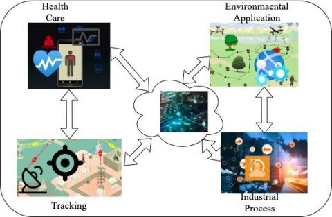
For different purposes, a WSN may be used as depicted in Figure 1; we may sum up few applications that are beneficial are as under:
a. Monitoring of habitat: Surveillance is a typical use of WSN, it is deployed in area monitoring from which some phenomenon is under surveillance. Vietnamize military is the best example in which the intruders were monitored after some periodic interval to check enemy intrusion. Similarly, WSNs can be used to detect the presence of vehicles in a parking slot.
b. Weather monitor: Word Environmental Sensor Networks have grown to check many earth science research applications of WSNs, which can be sensing of oceans, glaciers and forests of volcanoes.
c. Fire detection: In a forest, a network of nodes is to be mounted for detection of fire. This network can be fitted with sensors for measuring the humidity, gases and temperature in the trees or vegetation that are created by fire. Recently fire in Australian forests was also detected by the sensor nodes.
Data-Logging: For collection of data, surveillance of environmental information WSN is used. E.g., in a refrigerator monitoring of temperature, in nuclear power plants amount of water in overflow tanks are measured by these sensors.
Figure 1. Overview of WSN applications
As described above, the implementation of Wireless Sensor Network (WSN) technology will support a broad range of applications from habitat monitoring to battlefield surveillance [2, 3]. Few benefits include fast deployment, high fidelity sensing, low cost, WSN self-organization, and several other advantages. Despite many opportunities provided by the WSN, the technology also poses significant challenges. These problems are related to features of WSNs, namely:
In WSN, QoS is related to components like application part as well as user part. The WSN’s nature is different from the traditional networks. that make WSN’s quality of services QoS is still emerging area in research
1.2 Contribution of the paper
Wireless sensor nodes sometimes behave abnormally due to some conditions. The faults degrade the performance of the network which leads to be a serious issue. Therefore, key objective of our work is that it does the detection of the faults. Main contribution of this work is as under:
1.3 WSN architecture
A WSN consists of multiple wireless sensor nodes capable of data processing, communication with other sensor nodes and data storage. Because of its performance and cost-effectiveness, the WSN has gained wider applicability. Most WSN applications are related to monitoring and sensing of the environment. The sensing activity of the sensor nodes is achieved by the implanted microcontroller and radio transceivers. The microcontroller includes memory and processor, which enables the sensor node to perform simple computation and store the sensed data. Though the wireless sensor nodes can operate on its’own, sometimes the nodes need to communicate with other nodes. The communication between sensor nodes is achieved by the radio transceivers. The sensor nodes can sense the environment, process and forward the sensed data. There are two ways in which the communication between sensor nodes is done, which are direct and indirect. The connection includes two essential bodies, and they are the nodes of source and destination. The source node aims to forward the data to another node. The destination nodes are data receivers. Direct communication (or single-hop communication) is only possible when the receiving node lies in contact range of source nodes. If receiving node will not be within the source node’s range of communication, then the data is forwarded by using the intermediate nodes. If the receiving nodes are not in the communication range of source nodes, then data are forwarded by these intermediate-nodes that are further transferred to destination node. This is called indirect contact (or contact over multi-hop). With insufficient energy source, the sensor nodes are heavily constrained. The wireless sensor nodes are often deployed in hostile conditions, where removing or recharging batteries is not practical. The usable energy of the sensors must therefore be used effectively to maximize the lifespan of the sensor network. In the event that the sensor node does not effectively use the energy, its energy is depleted and contributes to node death. A nominal-energy sensor could serve its purpose. For instance, one sensor node's radio subsystem consumes more energy. Then it is easier to turn the radio on, only when the node has to communicate. Likewise, the sensor nodes have so many ways of saving resources. During transmission, the aggregation of data which is to be transmitted from different nodes into the sink-nodes is very expensive, that causes the congestion in WSN [4]. Fault diagnosis approaches are being utilized for the better control of sensor network that improves bandwidth and data reliability. Nonetheless, node energy efficiency increases with the use of the complicated methods for detecting faults. The fundamental objectives of sensor networks being reliability, cost efficiency, accuracy, versatility, and ease of deployment but sensor node failure can affect the accuracy and QoS [1]. WSN's general fault categorization is as: a) Software fault b) Hard fault. It is very difficult to separate the causes of these faults. Hard fault occurs due to failure of sensor module communication, sensor motion & energy loss and defective connections. Hard fault affects sensor nodes and connections that do not interact with their environment. In network cases, random noise errors cause damage to working devices, and defective transceivers cause software faults. Software faults are classified as (a) transient fault, (b) intermittent Fault, and (c) permanent fault.
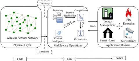
Incorrect detecting of an event or state at the middleware- layer is an error. An error is impact which results in faults sometimes. This considers a progressively serious issue with the gadgets since they are alive however detecting inaccurately. For instance, service crashes because of defective activity of services like detecting inaccurate context, and wrong construing; because of that event incitation isn't effectively happened, which conceivably prompts the disappointment of an application. For example, different sensors have been utilized to recognize a client in a smart house [5]. At the point, the person gets back home; the framework is then set according to the users inclinations. Unsuccessful attempt to accurately distinguish the user can bring about an unexpected framework setup. In any gadget, fault can prompt the unseemly control. Suppose inaccurate measuring of temperature readings would lead to over-cooling or overheating in that particular hall. Context info is utilized to adjust the surrounding to address user requirements. Figure 2 shows a usually observed faults order at physical layer in WSN applications [6]. So, for the successful operation of the network, early fault detection is highly needed. The foundation for progress lies in the capacity to draw significant and exact deductions from the gathered information, which thus requires having high sensor information. Software reliability in this manner is biggest concerns. So, we must design one of the efficient algorithms that will be utilized to recognize WSN software faults.
Figure 2. Generic architecture of sensor network applications
To manage these kinds of faults, two main parts like (I) distributed and (II) centralized way can be organized as WSN fault detection models, which can be further classified into various types as shown in the Figure 3. Such methods may cause large and rapid depletion of node energy which are closer to the center that causes some constraints in the network.
Figure 3. Classification of fault diagnosis
1.4 An overview of types of faults
The brief introduction about the types of faults:
Due to applications of wireless nodes in diverse conditions, these sensors are susceptible to failure and may lead to the overall failure of whole network. Software and hardware faults decrease overall efficiency of the WSN & therefore may impact deployment of the nodes. So, there comes the need for the diagnosis of such faults. By using either the multiple hops or single hops that follow protocol of MAC-layer. The communication process performed by the faulty sensor nodes will make the whole network to act faulty. Thus, to overcome this we can use intermittent faults as one of the main types of the software fault.
The WSN are the inherently fault-prone where reliability is mainly influenced by faults. Actually, a fault is malfunction in a system or an unexpected deviation, although it might not lead to of physically failure or breakdown. It can occur by different reasons, few are here like as de-synchronization, battery exhaustion, dislocation, radio interference. In general, we have found that the classification of faults is done on the basis of their duration, on their underlying causes, or we can say how a component behaves after the occurrence of fault [7]. Duration of fault basis, we have classified them as intermittent fault, transient fault and permanent faults. The permanent faults of sensor node cannot change its needs to get replaced or repaired. Transient faults occur suddenly without any apparent intervention, whereas the intermittent fault recurs itself irregularly. Due to their unpredictable behaviors, the intermittent faults and transient faults are not easy to diagnose. For WSN, it is mandatory to be able to early detection of faults for maintaining the quality of service.
In software fault detection fault tolerance is a subject that is having numerous recommendations & studies. Therefore, it is not so easy to provide full review of the state of the art all in one article. Nevertheless, WSNs are given specific characteristics, which allow current fault taxonomies to be expanded or tailored to the nature of such networks. To the best of our knowledge, this paper presents the attempt in proposing a specific work on software faults for WSNs and derivation of QoS.
The most realistic approach for identification of faults in WSN is comparison-based fault diagnosis approaches. These are much effective in nature because of spatial correlation and temporal exits in data sensed by sensors.
For fault detection and correction in WSN, a distributed Bayesian algorithm (BAFD) was proposed [8]. In case of BAFD, exchange of the data with its neighboring nodes in order to gain event's statistical likeliness and is used to classify faulty nodes with loss ratio. Faults detection of algorithm is given in which each node is used for detection of any suspicious activity by using the correlation of time [9]. The algorithm has low overhead communication but does not take the effect of transient failure into consideration and has good detection accuracy.
Panda and Khilar [10] proposed a self-detectable distributed fault detection algorithm to detect the faulty sensor nodes such as stuck at zero, stuck at one, stuck at nonzero and random fault in sensor networks. Here, each sensor node collects data from the neighbors and then diagnose itself by using the Neyman–Pearson test.
A new fault detection framework named SBFD was proposed which is lightweight, accurate, and scalable [11]. The framework was implemented in a test-bed network. Extensive simulation using a variety of network parameters was performed to assess the method’s scalability but the method could not analyze the network behavior during network operation, including deduction of possible reasons for failures and evaluation of routing protocols.
These researchers have proposed a dynamic method for failure detection (SBFD) for WSN. The work, a lightweight in network packet tagging is used for failure detection uses the checksum (Fletcher) & computation of server-side network route. This algorithm detects failure of node and link etc., which works on analysis of packet data. This work was having the drawback as its protocols didn’t recognize the different fault types [12].
Tai et al. [12] proposed failure detections for cluster for adhoc wireless networks. Here in this protocol, it uses exchange of the heart beat messages for identifying the node and link failures by cluster-based architecture.
Lee proposed detection of fault protocol for WSNs, taking into account of permanent & intermittent faults in both the sensor node and also in channel that are for communication. For fault detection, nodes and links are compared with the adjacent nodes, redundancy process is to be done. This protocol requires better computation and isolation of faults [13].
Syed et al. proposed a work in which every sensor node training them by using Fuzzy inference framework & data from neighboring sensor nodes. In this very recent study, Fuzzy Interference System is used for the diagnosis of faults in WSN [14]. The existing literature on the analysis of the WSN faults clearly reveals that the previous work focuses on the attention towards particular methods and fault tolerance algorithms rather than on sketching a comprehensive WSN fault detection.
The fault diagnosis in WSN wherein the RNN uses sensor data from the neighbor and previous samples for learning process. Statistical methods are used for detection of fault and classification is to be done by neural network. There are few other approaches which can be used for simple statistical and probabilistic methods. All these faults can be identified using performance matching criteria.
Rate optimization for node level congestion is another scheme that is used to solve the congestion problem by avoiding the buffer overflow for each WSN node [15]. The main disadvantage of this technique is rate adjustment dependency. In addition, the overload of management messages is not considered in its design. An evaluation for WSN existing routing protocols to determine which protocol can provide a better QoS using parameters such as throughput, end-to-end delay, and packet loss is presented by Kaur and Kaushal [16].
The closely related research given by a researcher namely Ayadi [17] in which the transport protocol for data transferring for reliable data. The actual idea of this work is to propose the transport layer for handling the issues of congestion which degrades the QoS. Few short comings in this work are neglecting the few common QoS parameters like energy consumption, density and bandwidth utilization.
Here we have discussed the drawbacks of various techniques of fault diagnosis present in the literature.
N number of sensor nodes deployed in an area randomly in which senor nodes are all independent which are located by any localization mechanism or GPS is used. Here we have assumed that according to node positions sensor nodes are using transmission of data by using single hop or multi-hop. Data history of readings is saved of k readings, in which k is a variable dependent on the type of quantity sensed by the sensor which is adjustable.
3.1 Proposed work
This work is mainly concerned for identification of faults in reading of data sensed by the wireless sensor nodes and also node failures. Fault identification of any sensor nodes can be done independently, as whenever sensor node finds its suspicious reading. We are assuming that initially sensor nodes Si, (i= 1, 2, 3. . . N) are free from fault & here the variable is "Normal ". The life span of each node during the process is in one status “Normal” or “Fault". The node is said to be Doubtful when fault diagnosis is to be processed and have not been yet confirmed "Fault" or "Normal". To find a Doubtful reading, each nodes are calculating the variations v of the past k readings where that sensed readings are to be stored and difference between the readings of sensor are Si. The node is considered as Doubtful if the time t and t-l is greater than the variation v. The condition can be given as:
$\begin{equation}
\left|X_{i}^{t}-X_{i}^{t-1}\right|>\min \left\{\sigma_{k}^{2}+x t h \pm x d r f t\right\}
\end{equation}$ (1)
where, $\begin{equation}
\sigma_{k}^{2}
\end{equation}$ is the variance of k readings, $\begin{equation}
X_{i}^{t}
\end{equation}$ is sensor nodes Si reading at time t. $\begin{equation} x d r f t\end{equation}$ is the difference in reading. Value of variance is given as:
$\begin{equation}
\sigma_{k}^{2}=\sum_{j=0}^{k}\left(x_{i}^{j}-\mu k\right)
\end{equation}$
Here, μk is mean of k readings.
$\begin{equation}
\mu k=\sum_{j-0}^{k-1}\left(x_{i}^{t-j}\right)
\end{equation}$
While a node Si finds a doubtful reading in a network it is broadcasting a message MessageBroadcast (t,CODi , $\begin{equation}
X_{i}^{t}
\end{equation}$) . Here t = timestamp, CODi is coordinate of node.
$\begin{equation}
X_{i}^{t}
\end{equation}$ is the reading of the sensor node at time t, these readings are spatially and temporally correlated but in a particular range. The nodes received the message, the measurement of sensor is correlated within a range “Rang.”, MessageBroadcast(t,CODi , $\begin{equation}
X_{i}^{t}
\end{equation}$) at a distance dist.
If the distance is beyond the range then discard this.
At sensor Sj which is in range dist. therefore the distance of the readings is equal to:
$\begin{equation}
\Delta X_{i j}^{t}=\min \left\{\left(\frac{D-d_{i j}}{d}\right) \times \mid X_{i}^{t}-X_{j}^{t}\right\} \pm X d_{r f t}
\end{equation}$
here, dij is Euclidian Distance between two sensor nodes.
dij= Si-sj
$\begin{equation}
\Delta X_{i j}^{t}
\end{equation}$ is the difference of Readings.
Every node which will receive the message will calculate the $\begin{equation}
\Delta X_{i j}^{t}
\end{equation}$: and will reply a message with the status of Message Broadcast (t, CODi, $\begin{equation}
X_{i}^{t}, \text {Status}
\end{equation}$) where a decision will be taken on it. As this work is proactive that means diagnosis will start automatically when any node is doubtful. After a particular interval, if the fault diagnosis starts then most of the nodes at interval generate a lot of traffic which exhausts the energy and the network throughput is degraded. Then because of this the proposed work do the diagnosis of fault process should affect nearby area nodes which finds itself doubtful. But in a case where most of nodes are doubtful and starts diagnosis on the same time, such situation can occur due to abrupt change in atmosphere like forest fire etc. In this case, network will identify the event occurrence and then report to the sink. It is not desirable that fault diagnosis degrade the performance of the network by flooding too much traffic at the same time. Therefore, the diagnosis process of faults should be executed in a way that throughput during this process would be unaffected or we can say less affected. For this issue to overcome we are using a window which works on time factor, because if all the doubtful nodes will be diagnosed on the same time that will cause power depletion, if it will work on the time stamp it will depend on the time expiry of selected time. As of random selection of nodes the probability of selecting same waiting time by all sensor nodes is very less. Therefore, all nodes start the diagnosis process at different time and generate comparatively smooth traffic in the network.
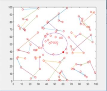
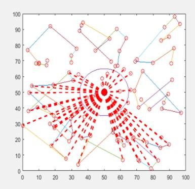
For identification of faults, we have designed five different scenarios given below:
(a)When no one node is faulty
(b) when only one sensor node is faulty
(c) when more than one sensor node is faulty
(d) abrupt reading change within a specific area
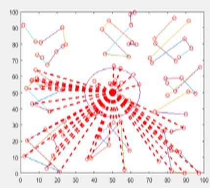
(e) if maximum number of nodes are faulty in non-faulty node area shown in figure
Figure 4. Illustration of faults occurs in specific regions
Procedure all above will handle as:
a. Initially all nodes have status“Normal”.
b. If $\begin{equation}
\left|X_{i}^{t}-X_{i}^{t-1}\right|>\min \left\{\sigma_{k}^{2}+x t h \pm x d r f t\right\}
\end{equation}$ then status of node is doubtful and it will be selecting a random timer value.
c. In the whole network when timer of node expires, a message will be broadcasted MessageBroadcast(t,CODi, $\begin{equation}
X_{i}^{t}
\end{equation}$).
d. Then node will find the difference of the reading and is given as
$\begin{equation}
\Delta X_{i j}^{t}=\min \left\{\left(\frac{D-d_{i j}}{D}\right)\right\} \times\left|X_{i}^{t}-X_{j}^{t}\right| \pm X d_{r f t}
\end{equation}$
e. A table (Tab) of nodes will be maintained of size ni.
f. once the nodes are getting the respond table is updated.
g. A for loop will be implanted.
if status
if (Tabstatus = =0) Increment;
Else-if (Tabstatus = =1) Increment;
Else-if (Tabstatus = =2) Increment;
Else-if (Tabstatus = =3) Increment;
Else (Tabstatus = = 4)
For i=1 to n
{
S(i) = sxi;
S(i) = syi;
Scenario1= Scenario2= Scenario3= Scenario4= Scenario5=0;
If Scenario0 >=5
(Status =”Normal”);
Break;
Else-If Scenario1 >=5
(Status =”Faulty”);
Break;
Else-If Scenario0 >=5
(Status =”Doubt”);
Break;
Else-if
MessageBroadcast(t,CODi , $\begin{equation}
X_{i}^{t}, \text {Status}
\end{equation}$ )
}
h. If the status is not updating consider it as Permanent fault.
3.2 Proposed algorithm
As we have states that is state‘x’. It can be like permanent faulty, fault-free, and intermittent faulty.
Algorithm
Node measurement of sensed data at discrete time DT.
Initialize P = 0 and Q = 0.
Data sensed with interval T & executed at different phase.
Detection phase:
Run detection phase.
If state ‘x’ is faulty & fault is detected, i.e., Q = 0 then
Waiting:
Set Q = 1.
end if
Observation stage:
Repetition of Loop
if state ‘x’ is faulty then
Counter = 0, r = 0.
if intermittent fault disappearance duration ≤ Expected fault duration of intermittent faulty node n−1 then
Incrementation ξ, i.e., Q = Q + ξ.
else
M = M + 1.
end-if
else
Incrementation of counter M = M + 1.
end if
if M > Threshold i.e. θ1 & Q < threshold θ2 then
Restart the Node, Set Q = 0 and M = 0.
else
Isolation is to be done.
end if
until Faulty Node Removal done.
For the software permanent fault, the range for the rate of fault is δp1 = 0.90 and δp2 = 1.10 and for the intermittent fault δin1 = 0.40 and δin2 = 0.89 while as for the transient fault the value of δtr1 = 0.02 and the value for δtr2 = 0.31.
Calculate Cfi = ∑r-1
If δp1≤Cfi ≤δp2 then
It can be permanent Soft fault
else if δin1≤Cfi ≤δin2 then
ni intermittent Faulty node
else-if δtr1≤Cfi ≤δtr2 then
ni can be Transient
else
ni can be fault free;
end-if
3.3 Design of proposed work
if(small>ma(i,3) && flag(ma(i,2))==0) small=ma(i,3);
pos=ma(i,2);
end
end
if pos==0 break; end
m=m+1; flag(source)=1; source
pos
small plot([Xpos(source),Xpos(pos)],[Ypos(source),Ypos(pos)]); source=pos;
l=((source-1)*(N1-1))+1;
%grid 2 % figure (1)
for i=N1+1:2*N1
Xpos(i)=Xm+rand*Xm; Ypos(i)=rand*Ym; AreaCode(i)=2; ENode(i)=Eo; plot(Xpos(i),Ypos(i),'or'); hold on;
end
source=11;
k=1;
for j=N:2*N1
if(i==j) continue;
else ma(k,1)=i; ma(k,2)=j;
ma(k,3)=sqrt(abs((power(Xpos(i)-Xpos(j),2)-power(Ypos(i)-Y pos(j),3))));
End
End
for i= l:l+N1-2 if(ma(i,1)==source)
if(small>ma(i,3) && flag(ma(i,2)-90)==0) small=ma(i,3);
end end
end
if pos==0
break;
end
m=m+1;
flag(source-90)=1;
source
pos
for j=1:2
for i=1:100 p(1)=plot(xunit(i),yunit(i),'o','MarkerFaceColor','r','Color','r'); pause (0.3)
delete(p(1)); %p(1)=plot(xunit(i)+i,yunit(i),'o','MarkerFaceColor','y','Color','y');
end
for i=2:200
disp(Xpos(i))
disp(Ypos(i)) end
for i=1:200
x_new(1)=Xpos(101);
y_new(1)=Ypos(101);
x_new(2)=Xpos(i);
y_new(2)=Ypos(i); line(x_new,y_new,'Color','r','LineStyle','--','linewidth',2); pause(0.4);
y(i)=x(i);%packets transfered
hold off;
end %sum
For evaluation of the proposed work, we have used simulator like MATLAB, NS2 where nodes were randomly distributed for simulation scenario. Fault detection algorithm simulation is computer based. Various parameters on which we have worked on are: In a range of transmission the number of sensor nodes is based on thresholds. For the best performance results the two thresholds, θ1 and θ2, need to be carefully chosen.
Network is simulated for near to 30 times for getting the results which are to be recorded and evaluated. For all sensor nodes we are assuming that the distance for correlation is taken as 105 m and transmission range of 70 m is to be taken. For our work we are going for accuracy for detection of faults, Network Throughput and number of messages needed for faults diagnosis.
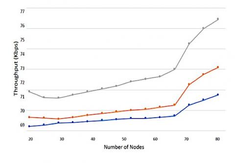
For comparison analysis we are doing a comparison of our proposed work with previous work which is designed by Wang et al. i.e., FDS [7]. Here we are analyzing the network throughput as shown in Figure 5. The throughput of network is first recorded by using protocol of routing which is a loop-free routing protocol know as Ad-hoc On-demand Distance Vector without using any mechanism of fault detection. Aftermaths we are checking throughput which is being monitored for both proposed and FDS work on the same network.
Figure 5. Number of wireless sensor nodes against the throughput of whole network
4.1 Network throughput diagram
In the NTD, during fault detection our proposed work maintains nearly the same throughput of the network. In the diagram below, proposed work is hardly affecting the system throughput. The throughput of network is very high as compared to previous work as because of management of network system divides the WSN in different groups. Every group have a well-defined area as the result proves this claim. In our work the fluctuations are of throughput is negligible as because of our management of systems. The expectation of throughput will be gradually increasing if the number of nodes get increased.
4.2 Accuracy of fault detection diagram
A higher fault detection accuracy in WSNs leads to higher fault-tolerance and consequently higher reliability. Diagram of accuracy of fault detection with respect to the failure rate is demonstrated as below:
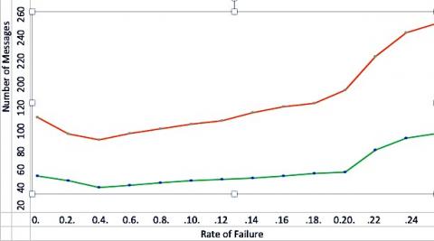
The Figure 6 shows fault diagnosis in the communication of network. It is clearly shown that work which we proposed is not communicating lot of messages in order to diagnose faults with number of faults.
With number of faults the communication of messages in both of the cases is only gradually increasing.
Figure 6. No. of messages verses rate of failure
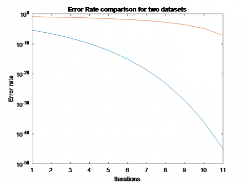
Figure 7. Error rate comparison for the two datasets
Figure 8. Error rate for two datasets
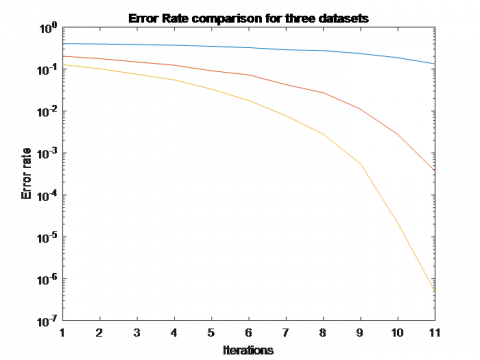
Figure 9. Error rate comparison for three datasets
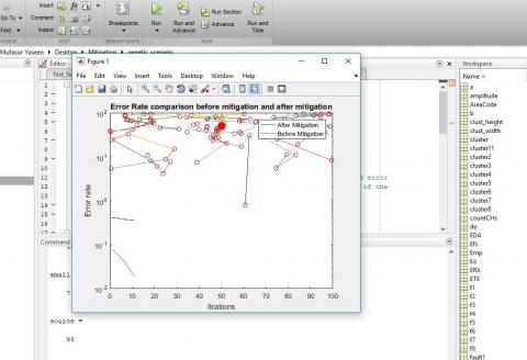
Figure 10. Error rate comparison before mitigation and after mitigation
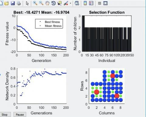
Figure 11. Best fitness & mean
After doing the simulation in order to mitigate the faults in which the error rates after doing the comparison in datasets that is shown in Figures 7, 8, 9. The error rates are minimizing after every iteration which enhances the QoS performance of our designed algorithm under an extended fault model. Especially we have focused on the case where the QoS in network is enhanced. In addition, due to the change in the fault model, a lower h1 results in better performance as expected. Moreover, it can be seen that the error rate is drastically reduced after the mitigation of the faults, thus making the network more error prone. This can be illustrated in Figure 10. Figure 11 is giving the best mean and fitness of network density, rows and columns shows here proper scenario.
In this work, we had discussed the state of art techniques for software fault detections in WSN & gave updated faults categorization techniques. The completeness of the fault diagnosis system is said to be achieved if sensor nodes could be diagnosed accurately by the fault detection computations along with the derivation of quality of services (QoS) like throughput etc. The full procedure for the analysis of faults is presented in this paper with different phases.
In future work, we can extend our work to various different applications of real-life and also for IoT-devices with different wireless sensor multi-functional networks so that we will achieve operability in the networking applications.
In the previous work, we found a few shortcomings by doing the analysis of detection techniques of software faults in WSNs. For future research, from the study we summarized the areas which need attention are:
As one can surmise, the biggest challenge for QoS provisioning in WSNs is how to provide the desired QoS to users and applications and in the same time preserve energy of WSNs and consequently increase network lifetime and thus this paper presents the desired QoS and the desired applications and also the fault mitigation techniques.
I am very much thankful to Er. Syed Farah Naz and Dr. Gholam Reza, Islamic Azad University, Yazad Iran. They helped me a lot during the execution of work. I am cordially very thankful to them.
|
N |
number of nodes |
|
T |
time interval, s |
|
P, Q |
initialization points |
|
k |
total readings |
|
s |
Sensor node |
|
v |
Variation of readings |
|
COD |
coordinate of node |
|
d |
distance |
|
x |
state of a node |
|
M |
counter value |
|
Greek symbols |
|
|
ξ |
dimensionless, incrementation |
|
θ |
threshold |
|
δ |
range of fault |
|
$\begin{equation} |
variance |
|
Subscripts |
|
|
p |
permanent |
|
in |
intermittent |
|
tr |
transient |
|
i, j |
number for the sensor node |
|
k |
total readings |
|
t |
timestamp |
[1] Muruganandam, M., Balamurugan, D., Khara, D. (2018). Design of wireless sensor networks for IOT application: A challenges and survey. International Journal of Engineering and Computer Science, 7(3): 23790-23795.
[2] Zhang, Z., Mehmood, A., Shu, L., Huo, Z., Zhang, Y., Mukherjee, M. (2018). A survey on fault diagnosis in wireless sensor networks. IEEE Access, 6: 11349-11364. https://doi.org/10.1109/access.2018.2794519
[3] Waltenegus, D., Christian, P. (2010). Fundamentals of Wireless Sensor Networks: Theory and Practice. A John Wiley and Sons, Ltd. https://doi.org/10.1002/9780470666388
[4] Ni, K., Pottie, G. (2012). Sensor network data fault detection with maximum a posteriori selection and bayesian modeling. ACM Transactions on Sensor Networks (TOSN), 8(3): 1-21. https://doi.org/10.1145/2240092.2240097
[5] Warriach, E.U., Kaldeli, E., Lazovik, A., Aiello, M. (2013). An interplatform service-oriented middleware for the smart home. International Journal of Smart Home, 7(1): 115-141.
[6] Warriach, E.U., Tei, K., Nguyen, T.A., Aiello, M. (2012). Fault detection in wireless sensor networks: A hybrid approach. 1st International Conference on Information Processing in Sensor Networks IPSN ’12, pp. 87-88. https://doi.org/10.1145/2185677.2185690
[7] Wang, Z.X., Wen, Q.Y., Sun, Y., Zhang, H. (2012). A fault detection scheme based on self-clustering nodes sets for wireless sensor networks. IEEE 12th International on Computer and Information Technology (CIT), Chengdu, China, pp. 921-925. https://doi.org/10.1109/CIT.2012.190
[8] Nitesh, K., Jana, P.K. (2015). DFDA: A Distributed Fault Detection Algorithm in Two Tier Wireless Sensor Networks. In: Satapathy S., Biswal B., Udgata S., Mandal J. (eds) Proceedings of the 3rd International Conference on Frontiers of Intelligent Computing: Theory and Applications (FICTA) 2014. Advances in Intelligent Systems and Computing, vol 328. Springer, Cham. https://doi.org/10.1007/978-3-319-12012-6_82
[9] Sharma, K.P., Sharma, T.P. (2017). rDFD: Reactive distributed fault detection in wireless sensor networks. Wireless Networks, 23(4): 1145-1160. https://doi.org/10.1007/s11276-016-1207-1
[10] Panda, M., Khilar, P.M. (2015). Distributed Byzantine fault detection technique in wireless sensor networks based on hypothesis testing. Computers & Electrical Engineering, 48: 270-285. https://doi.org/10.1016/j.compeleceng.2015.06.024
[11] Kamal, A.R.M., Bleakley, C.J., Dobson, S. (2014). Failure detection in wireless sensor networks: A sequence-based dynamic approach. ACM Transactions on Sensor Networks (TOSN), 10(2): 1-29. https://doi.org/10.1145/2530526
[12] Tai, A.T., Tso, K.S., Sanders, W.H. (2004). Cluster-based failure detection service for large-scale ad hoc wireless network applications. In International Conference on Dependable Systems and Networks, Florence, Italy, pp. 805-814. https://doi.org/10.1109/DSN.2004.1311951
[13] Mahapatro, A., Khilar, P.M. (2014). Online fault diagnosis of wireless sensor networks. Central European of Computer and Science, 4(1): 30-44. https://doi.org/10.2478/s13537-014-0203-8
[14] Syed, M., Dubey, M. (2019). A novel adaptive neuro-fuzzy inference system-differential evolution (Anfis-DE) assisted software fault-tolerance methodology in wireless sensor network (WSN). In 2019 International Conference on Computational Intelligence and Knowledge Economy (ICCIKE), Dubai, United Arab Emirates, pp. 736-741. https://doi.org/10.1109/ICCIKE47802.2019.9004396
[15] Prabakaran, N., Shanmuga, B., Prabakaran, R., Dhulipala, V. (2011). Rate optimization scheme for node level congestion in wireless sensor networks. In Proceedings of the International conference on Devices and Communications (ICDeCom), Mesra, India, pp. 1-5. https://doi.org/10.1109/ICDECOM.2011.5738548
[16] Kaur, B., Kaushal, S. (2014). QoS based evaluation of routing protocols in WSN. Proceedings of the IEEE Recent Advances in Engineering and Computational Sciences (RAECS), Chandigarh, India, pp. 1-7. https://doi.org/10.1109/RAECS.2014.6799501
[17] Ayadi, A. (2011). Energy-efficient and reliable transport protocols for wireless sensor networks: State-of-art. Journal of Wireless Sensor Network, 3(3): 106-113.