Mario A. Cucumo | Vittorio Ferraro* | Antonio Galloro | Daniela Gullo | Dimitrios Kaliakatsos | Francesco Nicoletti
OPEN ACCESS
Air coolers in an industrial plant are often a fundamental device to guarantee optimal conditions for processes. Evaporative air coolers are used to cool an air flow through the injection of water. They are also used to cool water in industrial process. They exploit a closed and pressurized circuit which implements cooling by forced exchange with air. In this paper the Computational Thermo-fluid Dynamics has allowed to evaluate the performance of evaporative cooling provided by the use of a water spray system. The analyzes allowed to study and identify the optimal configuration according to different parameters. The aim is to find out the arrangement that provides higher efficiencies. Configurations analysed differ from each other for droplet size, nozzle arrangement and air velocity. In the CFD analysis, the Discrete Phase Model is used to simulate the water injection on the continuous phase, represented by the air. In this way, heat transfer for droplet evaporation can be evaluated. This knowledge is crucial for designing efficient spray cooling systems. In addition to the efficiency improvement, correctly dimensioning an air cooler involves considerable advantages. In fact, other objectives obtained concern saving of water, necessary for example in arid areas, and the reduction of costs.
air cooler, water spray system, CFD simulation, evaporative cooler, droplet size, nozzle arrangement
This work represents an update of the previous paper on the parametric evaluation efficiency of evaporative cooler [1].
The study of different configurations of air cooler will be carry out through thermo-fluid dynamics simulations, realized by the software ANSYS [2]. Computational Fluid Dynamics can be a valuable tool for estimating the potential and the performance of evaporative cooling by water spray system.
In water spray cooling, water is sprayed into the inlet air in order to reduce the inlet air temperature by evaporative cooling. Cooler inlet air means better heat exchange for the air-cooler. In this way increases the overall system efficiency and helps the plant to recover some of the performance reduction caused by hot ambient temperatures. Evaporative cooling technologies are a smart way of air cooling in hot weather and in temperate climates [3].
An efficacious water spray design has to avoid non-uniform cooling distribution and incomplete evaporation of droplets. These issues can be avoided, and an optimum design can be achieved, only if the spray cooling mechanisms under these conditions is well understood. Spray cooling systems performance have been a subject of research for many years and many experimental studies and numerical models have been carried out [4-7].
Spray cooling performance is influenced by air velocity, nozzle arrangement, cone angle, injection rate, droplet velocity, injection direction and droplet size [8, 9].
Montazeri et al. [10] presented a systematic evaluation of the Lagrangiane-Eulerian approach for evaporative cooling provided by the use of a water spray system with a hollow-cone nozzle configuration. The evaluation was based on grid-sensitivity analysis and validated using wind-tunnel measurements [10]. Their study showed that CFD simulation of evaporation by using the Lagrangiane-Eulerian (3D steady RANS) approach, in spite of its limitations, can accurately predict the evaporation process with an acceptable accuracy. The local deviations from the wind-tunnel measurements were within 10 % for dry bulb temperature, 5 % for wet bulb temperature and 7 % for the specific enthalpy. The average deviations for all three variables were less than 3 % in absolute values.
Another experimental investigation on water spray for cooling tower application was conducted by Abdullah et al. [11]. The authors made use of open-circuit wind tunnel to simulate NDDCT built at the University of Queensland (QU). The phase dropper particle analyser was employed to characterize water spray. The study showed that low air velocity or small droplet size distribution are beneficial for cooling performance. The reason is that both droplet size and air velocity determine spray coverage that directly influences the spray cooling efficiency. Then the authors made a parametric analysis on the effect of different spray characteristics parameters, like droplet size distribution, injection velocities, spray cone angles and hollow-cone droplet size distribution patterns [12]. Considering an optimised nozzle and comparing this with a datum nozzle, it results around 15 % improvement in the spray cooling efficiency. Sun et al. conducted a study to evaluate the influence of injection direction on the spray cooler performance in a natural draft dry cooler tower [13]. The optimal injection for a hollow cone nozzle had been identified based on CFD study. This study shows that injection direction has a great influence on the evaporation process of the injected water droplets. For a single nozzle with the water mass flow rate of 5 g/s, the largest temperature drop is 1.27°C, corresponding to the radiator temperature of 38.73°C. Moreover, the increment of injection angle can enlarge the water-cooled area of radiators and the optimum injection angle varies with the height of nozzle location.
Sadafi and Hooman conducted a study with the aim to improve the knowledge base associated with the use of saline water in spray cooling applications [14]. Comparing saline water with pure water, it is obtained that saline water can improve cooling efficiency by 8% close to the nozzles. Moreover, full evaporation is achieved earlier compared to the pure water case. This accelerated evaporation process gives engineers the possibility to reduce the evaporation distance of up to 30 % from the nozzle exit.
Computational Fluid Dynamics can be a valuable tool for estimating the potential and the performance of evaporative cooling by water spray system [15]. It is important for the simulation to calculate, using psychrometric relationship [16], the mean parameters of the evaporative cooling process, such as outlet air temperature and humidity, water mass flow rate used for air-cooling and nozzle feed pressure.
Initial parameters known are volume flow rate and initial temperature conditions of the air, the desired final air humidity and the number of nozzles used to humidify, are showed in Table 1.
Table 1. Psychrometric calculation
|
va(m/s) |
Ta,i(°C) |
Ψa,i(%) |
xa,i(kgw/kga) |
Ta,o(°C) |
|
5.96 |
39.0 |
40.0 |
0.0176 |
29.07 |
|
Ψa,o(%) |
xa,o(kgw/kga) |
Qa(m3/s) |
${{\dot{m}}_{a}}$ (kg/s) |
n° nozzles |
|
85.0 |
0.0217 |
44.113 |
52.94 |
6 |
where, va is the inlet air velocity, Ta,i the inlet air temperature, Ψa,i the inlet air humidity, xa,i the inlet air specific humidity, Ta,o the outlet air temperature, Ψa,o the outlet air humidity, xa,o the outlet air specific humidity, Qa the air volume flow rate and ${{\dot{m}}_{a}}$ the air mass flow rate.
By mass end energy balance, it is possible to assume that the inlet air follows an isenthalpic process and the output point can be obtained from psychrometric chart. In fact, the final humidity of air is fixed and it is possible to calculate his enthalpy from initial condition of the air. Knowing final humidity and enthalpy it is possible calculate, in an iterative way, the final temperature and consequently the specific humidity. Another quantity that can be calculated, is the water mass flow rate the since the specific initial and final air humidity are known:
${{\dot{m}}_{w}}={{\dot{m}}_{a}}\cdot \left( {{x}_{a,o}}-{{x}_{a,i}} \right)$ (1)
where, $\dot{\mathrm{m}}_{\mathrm{w}}$ is the water mass flow rate. In this way, the water consumption can be calculated.
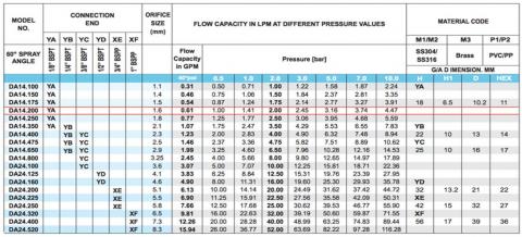
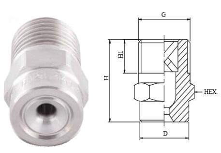
Once it has chosen the nozzle from constructor’s catalogue, it is possible to calculate the nozzle feed pressure as well. Nozzles manufactures provide a product technical sheet (Figure 1), which reports the volume flow rate and the corresponding feed pressure. So, on the basis of the water mass flow rate, it is possible to choose the nozzle to use and know the feed pressure. In this case, model DA14.200 is chosen. This nozzle allows to obtain, with a pressure p1=2 bar, a water volume flow rate equal to Q1=2 liters/min.
With the initial data of Table 1, the required volume flow rate per nozzle is equal to Q2=2.17 liters/min which corresponds a feed pressure of p2=2.35 bar, calculated by the relation below:
$\mathrm{p}_{2}=p_{1}\left(\frac{Q_{2}}{Q_{1}}\right)^{2}$ (2)
where, p1=2.0 bar and Q1=2.0 liters/min are the quantities indicated in the Figure 1.
Figure 1. Full cone spray nozzles data sheet
By controlling feed pressure in such a way, the water mass flow rate and thus the humidification rate can be varied.
The results obtained are indicated in the Table 2.
Table 2. Output data for nozzles
|
${{\dot{m}}_{w}}$ (kg/s) |
${{\dot{m}}_{w}}$/ nozzle (kg/s) |
${{Q}_{w}}$/ nozzle (liters/min) |
p (bar) |
|
0.217 |
0.0362 |
2.17 |
2.35 |
In this section a comparison between different air inlet velocities, nozzle arrangements, droplet size, and spray cone angle is conducted, in order to evaluate the better configuration, while other parameters are fixed in order to avoid to affect the results.
In a preliminary analysis is important to evaluate Reynolds number, that results equal to 1,250,000 and indicates a turbulent flow. In our case, the fluid involved is the air that we can consider incompressible because the Mach number is minor than 0.3, hence, pressure-based solver was chosen and the k-ε model was applied, in his realizable variant.
In order to simulate the system, it is essential to know a series of input data, for instance the inlet air temperature and mass fraction of water. Data of these simulations are taken from a real case and are shown in Table 1.
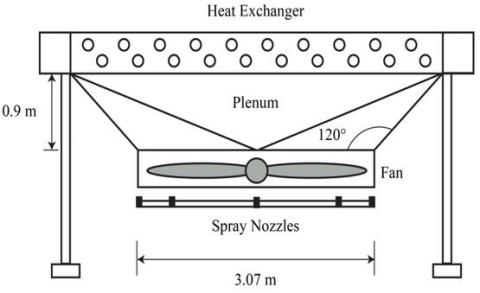
Final air humidity is the desired humidity that we want to achieve at the end of evaporative cooling process. A better situation occurs if saturated air is obtained, but in real applications this is impossible to be achieved. The causes are mixing time insufficient, exchange area not uniform and thus the air humidity doesn’t reach 100 %. If a further quantity of water is injected, it doesn’t evaporate but remains in the form of droplets. This could be a problem for fan blades corrosion and for the increased consumption of water. Therefore, manufacturers suggest 85 % as limit, on the basis of experimental results. This work refers to the air cooler shown in Figure 2, where the heat exchanger, fan, plenum and spray nozzles are highlighted. The simulations focus on the fan, spray nozzle and plenum section of the system.
Figure 2. Reference geometry of the air cooler
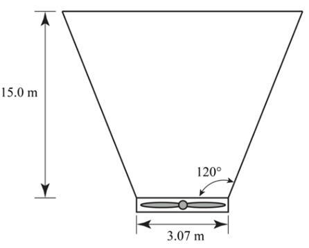
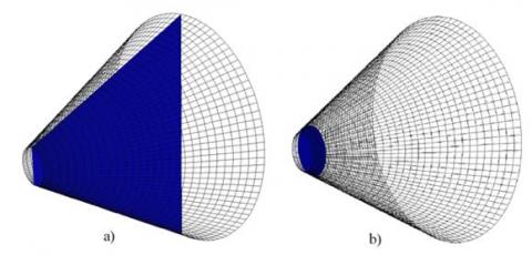
For computational reason, geometry will be slightly different with respect the real one. Computational domain is a truncated cone and its dimensions are shown in Figure 3.
Authors decided to extend the computational domain for the simulations to 15 m, in order to avoid the influence of the boundary condition on the solution, in the zone of interest.
Figure 3. Computational domain
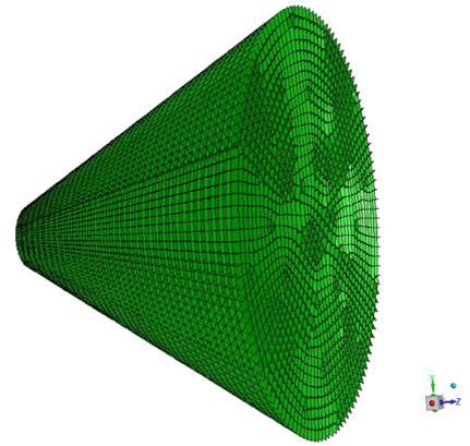
Mesh, for the computational domain, was created with the software GAMBIT of Fluent (Figure 4). The mesh created for the computational domain is composed by 49.630 cells. It is clear that calculation is quite computationally demanding. As you can see, no nozzles and fans appear in the computational domain, but these components were taken into account later.
Figure 4. Mesh for the computational domain
For the simulation, other data have to be set, and such data are the results of the psychrometric calculation carried out (Table 1) and reference geometry.
In order to simulate the motion produced by the fan, an angular component for the inlet velocity was set, evaluated from the fan technical sheet (Table 3).
Table 3. Fan technical sheet
|
Type of fan: AP (Manual Regulation) |
Type of fan draught |
Forced |
|
|
Nominal Diameter |
3048 mm |
Static pressure |
142.9 Pa |
|
Number of blades |
6 |
Volumetric flow rate |
44.03 m3/s |
|
Rotation speed |
212 RPM |
Fan blade material |
Aluminium |
|
Type of fan inlet |
Conical: L/D=0.15 |
Fan rotor material |
Aluminium or Carbon Steel |
For data concerning spray nozzle system, the first step is to choose number and type of nozzles. The calculation made refers to the model chosen in Figure 5, that is a full cone nozzle with an angle of 60°. In this work, different types of nozzle arrangements have been taken into account.
Figure 5. Full cone spray nozzle
3.1 Boundary conditions
The boundary conditions used are those of the wall, speed at inlet and outlet and pressure. The axial and angular velocity, temperature (312 K) and water mass fraction of the incoming air are set at the inlet.
At the outlet were set only air temperature (302.22 K) and air specific humidity (0.0217 kgw/kga). The goal is to investigate in which section the desired outlet conditions are achieved.
3.2 Discrete phase model
In addition to solving transport equations for the continuous phase, FLUENT allows to simulate a discrete second phase in a Lagrangian frame of reference. This second phase consists of spherical particles (which may be taken to represent droplets or bubbles) dispersed in the continuous phase. FLUENT computes the trajectories of these discrete phase entities, as well as heat and mass transfer to/from them. The coupling between the phases and its impact on both the discrete phase trajectories and the continuous phase flow can be included.
Authors decided to use Discrete Phase Model to simulate the water injection on the continuous phase, that is the air. In particular, droplet evaporation has to be evaluated. It can include a discrete phase in the FLUENT model by defining the initial position, velocity, size, and temperature of individual particles. These initial conditions, along with the inputs defining the physical properties of the discrete phase, are used to initiate trajectory and heat/mass transfer calculations.
The trajectory and heat/mass transfer calculations are based on the force balance on the particle and on the convective/radiative heat and mass transfer from the particle, using the local continuous phase conditions as the particle moves through the flow.
3.3 List of cases
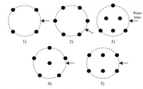
In this paper several cases have been studied, in order to compare them and find the best conditions. In particular different types of nozzle arrangement are simulated, as shown in Figure 6.
In addition, simulations were conducted for different air velocities, spray cone angles and droplet size, in order to assess their influence on the evaporative process (Table 4).
Figure 6. Different types of nozzle arrangement
Table 4. Values of the parameters used for the simulations
|
Air velocity |
2.0 m/s |
5.96 m/s |
10.0 m/s |
|
Spray cone angle |
30° |
45° |
60° |
|
Droplet size |
10 μm |
50 μm |
100 μm |
4.1 Grid- sensitivity analysis
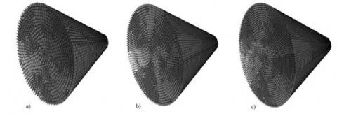
A grid-sensitivity analysis was performed based on two additional grids: A coarser grid and a finer grid. Grids are called M1, M2 and M3 and are composed by 24.948, 49.630 and 95.288 cells, respectively. Grids are shown in Figure 7.
Figure 7. Computational grids for grid-sensitivity analysis
The mesh independence was verified for the temperature profiles for two planes shown in Figure 8, named "Plane_0.9" and "Middle_Plane" respectively. Plane_0.9 is parallel to inlet plane and distant 0.9 m.
Figure 8. Planes for grid-sensitivity analysis: a) Middle_Plane; b) Plane_0.9
Mesh independence values are reported in Table 5. The results show a negligible dependence on the grid resolution. Therefore, grid M1 is used for further analysis.
Table 5. Mesh independence values of temperature
|
PLANE |
Middle_Plane |
Plane_0.9 |
|
M1-M2 |
0.10% |
0.37% |
|
M2-M3 |
0.05% |
0.61% |
4.2 Evaluation of cooling efficiency
Spray cooling system is mainly designed to humidify the inlet air, therefore, enhancing the performance of the air-cooler. In spray cooling system applications, cooling efficiency is generally considered as a good indicator in evaluating the performance of evaporative cooling systems. It represents how close the exiting air is cooled compared to the maximum possible temperature reduction (wet bulb temperature).
The cooling efficiency of a spray cooling system is defined as the ratio of the actual air temperature drop to the maximum possible temperature drop. Consequently, the global cooling efficiency can be expressed as:
${{\eta }_{c}}=\frac{{{T}_{db,i}}-{{T}_{db,o}}}{{{T}_{db,i}}-{{T}_{wb}}}$ (3)
where, Tdb,i, and Tdb,o are the dry-bulb temperatures of inlet and outlet air respectively, and Twb the wet-bulb temperature of the outlet air.
The global cooling efficiency defined as above and evaluated based on average temperatures at the inlet and outlet plane was used to investigate the performance of spray cooling system. Like outlet plane has been considered not the outlet plane of computational domain, but the “Plane_0.9”, that is the plane of interest (Figure 8).
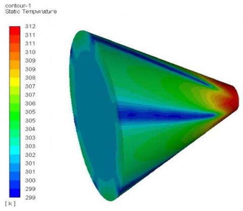
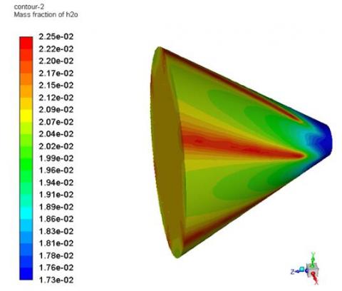
In the Figures 9 and 10 the distributions of the air temperature and water mass fraction in whole domain are shown for the nozzle arrangement 4.
Figure 9. Temperature distribution in whole domain for nozzle arrangement 4
Figure 10. Water mass fraction distribution in whole domain for nozzle arrangement 4
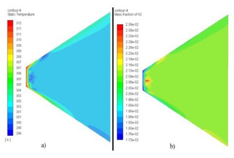
The evaporation along the computational domain causes the temperature of the droplets to reduce gradually and reach minimum values at the outlet of the domain. In fact, in Figure 11 temperature and water mass fraction distributions in the “Middle_Plane” can be clearly observed. An increase in water mass fraction corresponds in a decrease in air temperature due to evaporation. In fact, latent heat of vaporization is provided by air that cools because of this process.
Figure 11. Temperature and water mass fraction in the “Middle_Plane” for nozzle arrangement 4
4.2.1 Effect of nozzle arrangement on spray cooling efficiency
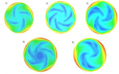
The different nozzle arrangements, shown in Figure 6 are compared, at the velocity of 5.96 m/s. In Table 6 are shown the cooling efficiency, the average air temperature and humidity in the “Plane_0.9”.
Table 6. Cooling efficiency, average air temperature and humidity for the five different arrangements in “Plane_0.9”
|
Nozzle Arrangement |
1 |
2 |
3 |
4 |
5 |
|
ηc |
65% |
69% |
69% |
71% |
68% |
|
T (K) |
304.2 |
303.7 |
303.6 |
303.4 |
303.8 |
|
Ψ |
74% |
78% |
78% |
80% |
77% |
As it can see, the better nozzle arrangement is the number 4 that allows a better distribution of the water flow and thus, a more efficient evaporation. In Figure 12 temperature contours of the different nozzle arrangements are shown. The nozzle arrangement 4 has the more uniform distribution of temperature, contrary to the nozzle arrangement 1. The vortex trend is due to the rotation provided by the fan.
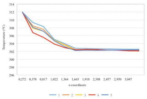
In Figure 13, it is reported the distribution of temperature in the “Middle_Plane”, considering average temperatures along the axis. This graph validates the results obtained from cooling efficiency calculation. In fact, the nozzle arrangement 4 has the best performance, because of its quickly drop temperature, in comparison to the others. On the contrary, the worst performance is of the nozzle arrangement 1, where the water mass flow is distributed between four nozzles rather than six. It obviously influences the evaporating area negatively, thus it needs more time to evaporate.
Figure 12. Temperature contours for the five different nozzle arrangements in “Plane_0.9”
Figure 13. Comparison of average temperatures in “Middle_Plane” for the five different nozzle arrangements
4.2.2 Effect of air velocity on spray cooling efficiency
Air velocity has a large influence on spray cooling efficiency and droplet transport. It affects droplet residence time (time that the droplets spend before the full evaporation or before reaching the outlet section, if not evaporated). Furthermore, it affects the droplet dispersion which influences the coverage area of the spray due to the momentum exchange. Considering the nozzle arrangement 4, cooling efficiency, average temperature and humidity in “Plane_0.9” are calculated for the velocities: 2.0, 5.96, 10.0 m/s, as shown in Table 7.
Table 7. Cooling efficiency, average temperature and humidity for different air velocities in “Plane_0.9”
|
Air velocity |
2.0 m/s |
5.96 m/s |
10.0 m/s |
|
ηc |
81% |
69% |
45% |
|
T (K) |
302.3 |
303.7 |
306.5 |
|
Ψ |
84% |
78% |
63% |
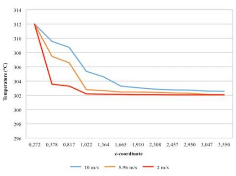
As expected, the spray cooling efficiency decreases as the air velocity increases, due to the residence time influence. Lower air velocity means longer droplet travelling time for the droplets. Furthermore, lower air velocity means larger coverage area because the time for droplets to lose momentum and follow the air stream is longer, which results in a better coverage area. Figure 14 confirms the results obtained: the drop temperature increases for lower velocities.
Figure 14. Comparison of average temperature in “Middle_Plane” for different air velocities
The spray cooling efficiency difference between 10.0 m/s and 2.0 m/s is more than double with respect to the one between 5.96 m/s and 10.0 m/s. The difference is due to the residence time difference. The droplet travelling time for air velocity of 10.0 m/s is more than double than that of 5.96 m/s whereas the residence time ratio between 2.0 m/s and 3.0 m/s is smaller. The average droplet residence time for 2.0, 5.96 and 10.0 m/s of air velocity are 0.57, 0.74 and 2.20 s, respectively, assuming that droplets follow the air flow immediately. Note that for velocity 2.0 m/s the air humidity is almost equal to 84 %, equal to the goal humidity.
4.2.3 Effect of spray cone angle on spray cooling efficiency
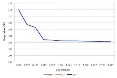
The influence of the spray cone angle is investigated by comparing the results for different half-cone angles, 30°, 45° and 60°. Cooling efficiencies, average air temperatures and humidity in “Plane_0.9” has been calculated for air velocity of 5.96 m/s and nozzle arrangement 4, and are reported in Table 8. The influence of spray cone angle is negligible, as confirmed by the results shown in Figure 15.
Table 8. Cooling efficiency, average air temperature and humidity for different spray angle
|
Spray angle |
30° |
45° |
60° |
|
ηc |
69.40% |
69.40% |
69.30% |
|
T (K) |
303.6 |
303.6 |
303.7 |
|
Ψ |
78% |
78% |
78% |
Figure 15. Comparison of average temperature for different spray angle in “Plane_0.9”
4.2.4 Effect of droplet size on spray cooling efficiency
Another important factor affecting spray cooling efficiency is droplet size. Small droplets provide more surface area per unit volume than large droplets and evaporation only occurs at the water/air interface. Evaporation rate per unit volume of droplets in gaseous media is related to the square of the droplet diameter and increases rapidly when droplet diameter is decreased.
The comparison is made fixing the air velocity (5.96 m/s) and for the nozzle arrangement 4. Table 9 shows the modified spray cooling efficiency, average temperature and humidity in “Plane_0.9” for different droplet diameter, 10, 50, 100 μm.
Table 9. Cooling efficiency, average air temperature and humidity for different droplet diameter in “Plane_0.9”
|
Diameter |
10 μm |
50 μm |
100 μm |
|
ηc |
69% |
54% |
46% |
|
T (K) |
303.7 |
305.6 |
306.4 |
|
Ψ |
78% |
67% |
63% |
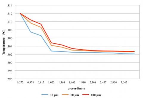
It is clear from this table that at the same air velocity, at smaller droplet diameter, more evaporation and consequently higher cooling is achieved. This behaviour is due to the fact that the total exposed water surface area between water and air flow is larger for sprays with smaller droplets. Therefore, the evaporation rate is higher. Figure 16 confirms the previous results.
Figure 16. Comparison of average temperature for different droplet diameter in “Plane_0.9”
The spray cooling efficiency difference between 10 μm and 50 μm is almost double than the one between 50 μm and 100 μm and this is due to the residence time difference. The droplet travelling time for droplet diameter of 10 μm is more than double with respect to that of the 50 μm diameter droplet, whereas the residence time ratio between 50 μm and 10 μm is smaller. The average droplet residence time for 10 μm, 50 μm and 100 μm of droplet diameter are 0.74, 2.66 and 3.07 seconds, respectively. This consideration confirms the smaller difference between the curve of 50 μm and 100 μm compared to those at 10 and 50 μm of droplet diameter, in Figure 16.
This work introduces a study conducted by Thermo-Fluid Dynamic simulation, in order to evaluate the performance of evaporative cooling, provided by a water spray system. Droplet evaporation and the resulting air cooling were studied, as a function of some parameters, like air velocity, nozzle arrangement, spray cone angle and droplet size. A cooling efficiency factor was introduced to evaluate the entity of cooling process.
Considering the nozzle arrangement reported in Figure 6, the best configuration is the number 4, because of its impact on the spray coverage area. Cooling efficiency value range is from 71 % to 65 % for the worst arrangement, the number 1. For the other configurations, values are very closer, 69 % for arrangements 2 and 3 and 68 % for arrangement 5. The final air temperature varies from 304.2 K for arrangement 1, to 303.4 K for arrangement 4. In the better case the temperature drop is equal to 8.6 K.
Changing air velocity from 2.0 m/s to 10.0 m/s, cooling efficiency decreases from 81 % to 45 %. It means that air velocity has a significant impact on cooling performance, because of its impact on residence time. In fact, final temperature increases from 302.3 K to 306.5 K that is a wide range. Air humidity reaches 84 % for air velocity of 2.0 m/s, the greater value obtained.
The angle of the spray cone has varied from 30° to 60° and the results indicate that this parameter has a negligible impact on cooling efficiency. In fact, the cooling efficiency is almost constant.
For the evaluation of impact of droplet size, last one was changed in a range from 10 μm to 100 μm. Cooling efficiency increases if droplet size decreases, for the influence on residence time. Cooling efficiency varies from 69 % to 46 % and final temperature from 303.7 K to 306.4 K. This impact is significant on cooling performance.
The results of this study confirm that such technology enhances the performance of a plant, built in arid areas, operating on existing devices, without high cost. In fact, we arrive to a temperature drop of 9.7 °C, and such result improve the heat transfer coefficient of the air-cooler, when ambient air temperature is very high.
The reported study shows that humidity in the better case is equal to 84 %, according to manufactures suggestions, so we can say that the results are quite accurate. To validate the results obtained, the authors intend to proceed with experimental measures.
${{\dot{m}}_{w}}$ Water mass flow rate (kg/s)
${{\dot{m}}_{a}}$ Air mass flow rate (kg/s)
p1 Initial pressure for nozzle (bar)
p2 Final pressure for nozzle (bar)
Qa Air volume flow rate (m3/s)
Q1 Initial volume flow rate for nozzle (m3/s)
Q2 Final volume flow rate for nozzle (m3/s)
Qw Water volume flow rate (m3/s)
Ta,i Inlet air temperature (°C)
Ta,o Outlet air temperature (°C)
Tdb,i Dry-bulb temperature of inlet air (°C)
Tdb,o Dry-bulb temperature of outlet air (°C)
Twb Wet-bulb temperature of the air (°C)
va Inlet air velocity (m/s)
x Specific humidity (kgw/kga)
xa,i Inlet air specific humidity (kgw/kga)
xa,o Outlet air specific humidity (kgw/kga)
Greek symbols
ηc Global cooling efficiency (%)
Ψa,i Inlet air humidity (%)
Ψa,o Outlet air humidity (%)
Subscripts
a Air
i Inlet
o Outlet
db Dry-bulb
w Water
wb Wet-bulb
[1] Cucumo, M.A., Ferraro, V., Galloro, A., Gullo, D., Kaliakatsos, D., Nicoletti, F. (2019). Computational fluid dynamics simulations to evaluate the performance improvement for air-cooler equipped with a water spray system. Tecnica Italiana - Italian Journal of Engineering Science, 63(2-4): 158-166. https://doi.org/10.18280/ti-ijes.632-407
[2] ANSYS Fluent 12.0, Theory Guide. (2009). ANSYS Inc.
[3] Costelloe, B., Finn, D. (2003). Indirect evaporative cooling potential in air-water systems in temperate climates. Energy Buildings, 35(6): 573-591. https://doi.org/10.1016/S0378-7788(02)00161-5
[4] Zhou, N., Chen, F., Cao, Y., Chen, M., Wang Y. (2017). Experimental investigation on the performance of a water spray cooling system. Applied Thermal Engineering, 112: 1117-1128. https://doi.org/10.1016/j.applthermaleng.2016.10.191
[5] Kachhwaha, S.S., Dhar, P.L., Kale, S.R. (1998). Experimental studies and numerical simulation of evaporative cooling of air with a water spray - II. Horizontal counter flow. International Journal of Heat and Mass Transfer, 41(2): 465-474. https://doi.org/10.1016/S0017-9310(97)00131-2
[6] Sureshkumar, R., Kale, S.R., Dhar, P.L. (2008). Heat and mass transfer processes between a water spray and ambient air - I. Experimental data. Applied Thermal Engineering, 28: 349-360. https://doi.org/10.1016/j.applthermaleng.2007.09.010
[7] Tissot, J., Boulet, P., Trinquet, F., Fournaison, L., Macchi-Tejeda, H. (2011). Air cooling by evaporating droplets in the upward flow of a condenser. International Journal of Thermal Sciences, 50: 2122-2131. https://doi.org/10.1016/j.ijthermalsci.2011.06.004
[8] Sun, Y., Guan, Z., Gurgenci, H., Li, X., Hooman, K. (2017). A study on multi-nozzle arrangement for spray cooling system in natural draft dry cooling tower. Applied Thermal Engineering, 124: 795-814. https://doi.org/10.1016/j.applthermaleng.2017.05.157
[9] Sun, Y., Guan, Z., Hooman, K. (2017). A review on the performance evaluation of natural draft dry cooling towers and possible improvements via inlet air spray cooling. Renewable and Sustainable Energy Reviews, 79: 618-637. https://doi.org/10.1016/j.rser.2017.05.151
[10] Montazeri, H., Blocken, B., Hensen J.L.M. (2015). Evaporative cooling by water spray systems: CFD simulation, experimental validation and sensitivity analysis. Building and Environment, 83: 129-141. https://doi.org/10.1016/j.buildenv.2014.03.022
[11] Alkhedhair, A., Guan, Z., Jahn, I., Gurgenci, H., He, S. (2015). Parametric study on spray cooling system for optimising nozzle design with pre-cooling application in natural draft dry cooling towers. International Journal of Thermal Sciences, 90: 70-78. https://doi.org/10.1016/j.ijthermalsci.2014.11.029
[12] Alkhedhair, A., Jahn, I., Gurgenci, H., Guan, Z., He, S. (2015). Water spray for pre-cooling of inlet air for natural draft dry cooling towers - experimental study. International Journal of Thermal Sciences, 90: 70-78. https://doi.org/10.1016/j.ijthermalsci.2014.11.029
[13] Sun, Y., Guan, Z., Gurgenci, H., Hooman, K., Li, X., Xia, L. (2017). Investigation on the influence of injection direction on the spray cooling performance in natural draft dry cooling tower. International Journal of Heat and Mass Transfer, 110: 113-131. https://doi.org/10.1016/j.ijheatmasstransfer.2017.02.069
[14] Sadafi, M.H., González Ruiz, S., Vetrano, M.R., Jahn, I., Van Beeck, L., Buchlin, J.M., Hooman, K. (2016). An investigation on spray cooling using saline water with experimental verification. Energy Conversion and Management, 108: 336-347. https://doi.org/10.1016/j.enconman.2015.11.025
[15] Blazek, J. (2001). Computational Fluid Dynamics - Principles and Applications. Elsevier Science Ltd. The Boulevard Langford Lane, Kidlington, Oxford OX5 IGB, UK.
[16] Wang, S.K. (2001). Handbook of air conditioning and refrigeration. McGraw-Hill, Two Penn Plaza, New York, NY 10121-2298.