Benabbou Amin* | Hamdadou Djamila
OPEN ACCESS
The aim of this article is to propose a solution to the problem of spatial data warehouses evolution over time. In addition to the difficulties encountered when working on the evolution of non-spatial dimensions, which have been the subject of many scientific articles, the introduction of space at the level of dimensions makes us confront, on one hand, to a modelling problem in which a set of zones forming a hierarchical mesh are subject to numerous territorial events, where it is a question of being able to find the configuration of the territory as it was at a given time. The second problem that emerges from this configuration is that of having to estimate the value of an indicator for a zone when the exact value is not known. Dimensions evolution is made possible thanks to the adaptation of the so-called implicit versioning technique to spatial data. To respond to the second problem, a spatial interpolation method based on the combined use of the map of agglomerations and the population of municipalities in the estimation procedure has been proposed. The proposed spatial interpolation method can be used in estimating the value of different health indicators.
epidemiological surveillance, spatiotemporal data warehouses, territory evolution, spatial interpolation, public health indicators
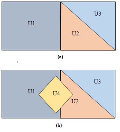
In a spatial data warehouse, the spatial dimension is often used to describe the territory; in this configuration, each level of this dimension proposes to divide the territory into a set of zones. Zones that make up the mesh of each level form a layer and are subject to numerous territorial events. This dynamic, when taken into consideration in a spatial data warehouse, poses a serious problem with respect to data exploration process where the system can be made to estimate the value of a measure to be assigned to a zone for a period for which this zone did not exist yet or to a zone whose shape has been altered compared to the current configuration. Figure 1 shows an example of a territory evolution between times T1 and T2. Version 2 of the territory was marked by the appearance of zone U4 at time T2. In this case, which measure value will the system assign to U4 at time T1? It should also be noted that even if this is a simple territorial event, the space required for the creation of U4 was taken from zones U1 and U2. So the same question arises for them when it comes to know the value of the measures to be assigned to them at time T1 using the version 2 of the territory.
In a more general context, dimensions, whether spatial or not, have always been considered as static, but examples from the real world show that they are subject to many changes. Dimension evolution is made possible thanks to the management of several versions of the warehouse where the content of each version is only valid for a certain period of time. In this configuration, a new version is created whenever a change or a set of changes that occur at the same time, affect the warehouse. Primarily, two concepts have been proposed to manage these versions: implicit versioning and explicit versioning.
Implicit versioning relies on adding extensions to the warehouse components that may change over time. These extensions relate to the addition of time validity intervals and the definition of transformation functions. Validity intervals are used to mark the validity periods of the various components of the warehouse (dimensions, facts, dimension levels, members, etc.). Transformation functions allow us to map dimension members between each two consecutive versions using weighting coefficients. In such a configuration, each version is seen as a selection of the warehouse components that are valid at a time t. [1] have proposed an approach which is based on this principle, but the temporal extensions have been attributed only to dimension members as well as hierarchical links between them. To avoid using the transformation functions each time a query is executed, the authors propose to compute these transformations in a previous step and to store the result in different data stores. A data store is dedicated to each version. In [2], the authors complement the work that has been done in [1] by proposing the COMET, a prototype that has the ability to intercept changes that can affect the structure as well as the instance of the warehouse dimensions.
In an explicit versioning, each version of the warehouse is stored in a separate database, so the system is linked to multiple databases at the same time. [3] proposed the concept of multi-version data warehouses. The developed prototype responds to changes that affect both the scheme and the content of the warehouse. In addition to the so-called real versions, which are created to respond to the changes affecting the data warehouse, the proposed approach manages a set of so-called alternative versions that are created for simulation purposes. To query the multi-version data warehouse, extensions have been added to the SQL language. [4] have extended the work done in [3] on multi-version data warehouses by proposing an improved version of the meta-model which used to ensure a good management of the different versions that make up the warehouse. A platform for automatic detection of changes that occur in external data sources and the generation of corresponding actions has also been proposed.
Figure 1. Territory states at times T1 (a) and T2 (b)
To our knowledge, only one work has addressed the question related to the evolution of spatial dimensions over time. It is the M3 model that has been proposed in [5]. In M3, the evolution of the territory is made possible at the level of spatial dimensions through the use of a regular grid that proposes to cut the surface of the territory into spatial entities that are time invariant. The aggregation of these entities forms spatial members, or zones, of the lowest level of the spatial dimension. Thus, calculating the value of a measure for a spatial member which results from merging two zones m1 and m2, for example, depends on the number of spatial entities that come from m1 and those originating from m2. This technique is easy to implement but dimension members weighting coefficients calculation is based on the strong assumption that the distribution of the measures is spatially uniform, which is generally false and is considered as an extreme simplification of the geographical reality [6], page 78. More generally, this problem looks as follows: we have an initial mesh, called source mesh, for which the exact value of the zone is known at the level of each zone that composes it. We also have another mesh, called target mesh, which represents the same territory as the source mesh but which proposes to cut it in a different way. Spatial interpolation is the term that has been assigned to all the techniques that aim to find an estimate of the value of each target zone indicator or variable using the source mesh. Three families of methods have been identified: surface-based spatial interpolation, point-based spatial interpolation and spatial interpolation based on the use of auxiliary data.
Surface-based spatial interpolation methods proceed to estimating the value of the indicator at each zone of the target mesh by superimposing the target mesh on the source mesh. The estimation is then made according to the area of the zones that result from the intersection between the two meshes with respect to the area of each target zone or with respect to the area of the source zones whose each intersection zone is derived. These methods are used without any problem in the case where the variable to be estimated distributes uniformly within each zone. Unfortunately, in practice, few variables obey this constraint.
Point-based spatial interpolation methods estimate the value of each target zone variable by superimposing a grid on the source mesh and applying a point interpolation method to estimate the value of each node present on the grid. Estimating the value to be assigned to each target zone c is done by calculating the average of the estimates of all nodes that lie within c. The fundamental problem of these approaches is the same as that of the point interpolation method which has been used in calculating node values, namely, the hypothesis made on the surface [7].
Spatial interpolation methods that are based on the use of auxiliary data are mainly used to estimate population density, but their use is not limited to that. The general principle of these methods is to exploit the knowledge that is available on the territory to identify, within each zone of the mesh, regions that have different population densities. The initial goal is to provide a more realistic visualization than traditional methods that affect a single value to each zone [8], page 84. Among the auxiliary data that have been used in the calculating the population density, we mention: the density of roads, the type of land use (urban area, rural area, industrial zone, etc.) and the intensity of the night light of cities. These methods have been used very little in estimating values of the epidemiological variables, and this for many reasons: “One reason for this limited interest is undoubtedly ignorance about their potential; others are perhaps suspicion about their reliability and a lack of the relevant skills and technologies for data manipulation” [9], page 395.
In this article, we will propose a solution to the problem of spatial data warehouses evolution. The evolution considered here concerns both the instance of non-spatial and spatial dimensions. On the one hand, the proposed solution will allow us to trace all the changes through which a set of hierarchically organized zones can pass. The aim is to be able to use any version of the territory for data exploration. Then, this solution will allow us to estimate the value of a measure that must be assigned to a zone when the exact value is not known. The estimate considered here concerns the number of Tuberculosis cases recorded within a zone.
The remainder of this paper is organized as follows: in the next section, we will present details of spatiotemporal data warehouses as we see them. We will first expose the mechanisms that have been used to adequately manage the evolution of the content of spatial data warehouses. Then we will address the question of calculating weighting factors in the case of spatial dimensions. In the third section, we will first present TUBERCOLAP, a SOLAP (Spatial On-line Analytical Processing) prototype, which we have developed and the data set that has been used to supply its warehouse. To make in practice the key concept of spatiotemporal data warehouses, namely, the evolution of the spatial dimension, a case study on tuberculosis screening at the level of department of the Tlemcen will be presented. Through this study, we will proceed to a brief description of the main changes that the administrative division of the department has known. Next, we will present the transformation matrices that emerge from calculating the weighting factors using the proposed method. The article will finish with a conclusion that will summarize the main points that have been discussed in this article and will draw up some perspectives.
In this section, we will present details related to spatiotemporal data warehouses as we see them. We will first explain the mechanisms that have been used to implicitly manage versions that make up the warehouse. Then we will address the question of calculating weighting coefficient for spatial dimensions.
2.1 Spatiotemporal data warehouses
A spatiotemporal data warehouse results from the enrichment of a spatial data warehouse through the introduction of temporal validity intervals at the level of the components that are likely to evolve over time, and the definition of the transformation functions which are needed to match the dimension members between each two successive versions (see Figure 2). These concepts have already been seen in implicit versioning (discussed in the introduction), however, the evolution considered here concerns both non-spatial and spatial members.
In order to minimize the human factor in upgrading the warehouse when it is affected by changes, we have chosen to restrict the scope of possible changes to those that affect its instance, it is why Validity intervals have been added to measures, level attributes, spatial and non spatial dimension members, and hierarchical links between members only.
Several authors have stressed the importance of separating the spatial component of the thematic component when it comes to follow the evolution of a spatial entity. The purpose of this separation is to allow the two domains, spatial and thematic, to evolve independently of each other (a municipality may change its name without its spatial extent being affected, or vice versa), this has the consequence of avoiding data duplication through sharing the components that remain intact. The principle of separation is materialized here at the level of zones thanks to the classes: Spatial Member which contains all the thematic attributes of the zone, and Spatial_Extension through which we can trace the history of all the changes of form by which the zone has passed.
Figure 2. Spatiotemporal data warehouses
The meta-model of Figure 2 is marked by the creation of the class Version, through which we keep track of all versions that the warehouse contains. Each version is only valid for a certain period, and is linked to the version that follows it and to the one that precedes it. The Version_Mapping relation class allows us to express the values of all the weighting factors. Concretely, the transformation functions take the form of a matrix [1, 2], called here the transformation matrix, which must be defined for the members of each dimension level, spatial or not, between each two successive versions to be able to explore data of the warehouse using the first version or using the second one.
Working with the example of Figure 1, mentioned in the introduction, the transformation matrix that must be defined between the two versions is shown in Table 1. For a zone that is located in version 2 of the territory and for which the exact measure value is not known, estimating this value is done by calculating the weighted sum of all the measure values of the zones of version 1 of the territory, this is equivalent to using the weighting coefficients that are in same column than the zone whose value is to be calculated. We proceed in the same way when it comes to estimating the measure value for a zone situated in version 1 of the territory, except that the weighting coefficients to be used are those that are in the same line as the zone whose measure value is to be calculated.
The management mechanism of the different versions that make up the spatiotemporal data warehouse is the same as that proposed in [2] which have been defined in the context of non spatial data warehouses. So, versions are stored as data marts, where each data mart contain all data of the warehouse but are organised according to the content of each version the data mart is representing. Data contained in each data mart are aggregated and are ready to be explored, so no extensions to the query language are needed. An analysis session starts by choosing the warehouse version to be used for exploring the spatiotemporal warehouse data, most of the time, it is the most recent version, but the system gives us the possibility to choose an older version as a basis for data exploration operations.
Table 1. Matrix of transformation defined between Version 1 and version 2
|
|
Version 2 |
|||||
|
|
|
U1 |
U2 |
U3 |
U4 |
|
|
Version1 |
U1 |
1-w1 |
0 |
0 |
W1 |
|
|
U2 |
0 |
1-w2 |
0 |
W2 |
||
|
U3 |
0 |
0 |
1 |
0 |
||
2.2 Weighting factors calculation for spatial members
In the case of non-spatial members, the value of each weighting coefficients, wi, is assigned subjectively according to the knowledge we have about the members who are involved in the different types of change. However, when dealing with spatial members, estimating the value of the measure that must be assigned to a zone when the exact value is not known is a problem whose solution depends necessarily on type of the indicator (or the measure) whose value is to be estimated. In domains where the value of the measure is uniformly distributed across the surface of the zone, the application of a surface-based interpolation method will produce very satisfactory results. However, in a domain such as tuberculosis screening, the number of recorded cases varies from one region to another even inside the same zone, because the exposure to tuberculosis is governed by several factors, such as population density, humidity level, etc. In this case, the application of a spatial interpolation technique that involves auxiliary data that are related to these factors will inevitably produce more realistic results.
Since the number of persons who are infected with tuberculosis in a zone is proportional to the density of its population, we have chosen to use the population as a weighting factor. In this context, only the population of zones that have not undergone changes is known. The technique used here can be seen as an adaptation of the binary method that has been proposed in [10] by:
Replacing the binary mask, obtained by the automatic classification of a satellite image pixels into inhabited and uninhabited pixels, with a vector layer containing all the agglomerations which lie within the territory where our study is taking place. The same agglomeration may belong administratively to several municipalities, so it is common to have an agglomeration, part of which is located inside a municipality and the other part inside another municipality.
Using the spatial interpolation method to calculate values of the weighting coefficients which, in turn, are used in estimating the number of people with tuberculosis in zones where the exact number is not known, and not to find, within a given zone, regions with different population densities as was the case in [10].
The weighting factors calculation is done according to the following algorithm:
Inputs:
Outputs:
Beginning
End.
Population(a)=$\sum\nolimits_{i=1}^p\frac{Asai}{Aai}*Population(si)$ (1)
Population (sc)=$\sum\nolimits_{j=1}^q\frac{Ascj}{Aaj}*Population(aj)$ (2)
wi =$\frac{Population(sci)}{\sum\nolimits_{j=1}^kPopulation(scj)}$ (3)
In Eq. (1):
p: is the number of source zones that partially include agglomeration a.
Asai: is the surface of the zone that results from the intersection of the source zone si with agglomeration a.
Aai: is the total surface of all agglomerations that are inside the source zone si.
In Eq. (2):
q: is the number of agglomerations that are wholly or partially inside the zone sc.
Ascj: surface of the zone resulting from the intersection of agglomeration j with area sc.
Aaj: surface of the agglomeration j.
In Eq. (3):
k: is the number of zones that result from the intersection of zone c with all zones of the source mesh.
To discuss the key concept of spatiotemporal data warehouses, namely, spatial dimension evolution, a case study on tuberculosis screening at the level of department of the Tlemcen has been done. In this section, we will first present TUBERCOLAP, a SOLAP prototype, which we have developed as well as the data set that has been used to feed its warehouse. Then, we will proceed to a brief description of the main changes that the administrative division of the department has known as well as the transformation matrices that emerge from calculating the weighting coefficients using the proposed spatial interpolation method.
3.1 Tubercolap
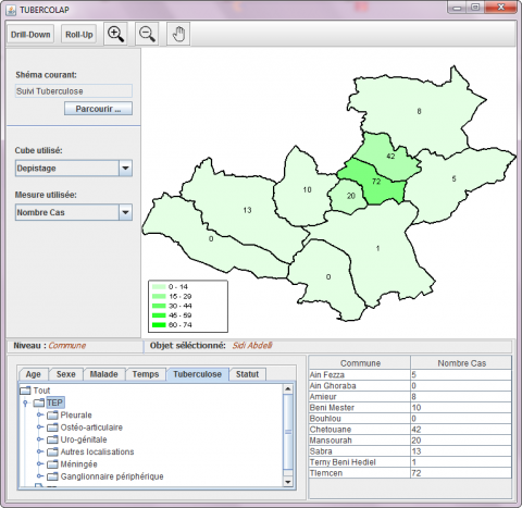
Figure 3. Tbercolap
Figure 3 shows the user interface of our prototype, TUBERCOLAP, which was developed to monitor tuberculosis screening results at the level of Tlemcen department. TUBERCOLAP is a SOLAP-type data exploration tool that is connected to a spatiotemporal data warehouse in which spatial and non-spatial dimensions can evolve over time. At the level of each department, tuberculosis screening aims to permanently recognize tuberculosis cases in all health services, in order to treat them with specific chemotherapy. The recorded cases are then analyzed according to the following axes:
Patient gender.
Patient age: the analysis is done according to two hierarchies: {0-14 years, 15 years or more} or {0-14, 15-24, 25-34, 35-44, 45-54, 55 -64, 65 and more}.
Tuberculosis type: pulmonary or extra-pulmonary.
Initial bacteriological status (results of direct saliva microscopy and / or macroscopic results of saliva after culture).
Patient type: New case, Failure, Relapse, Progressive resumption after interruption or Other.
3.2 Spatial dimension evolution
In the context of our study, the spatial dimension is organized according to three levels: Municipalities, Daïras and Health sectors:
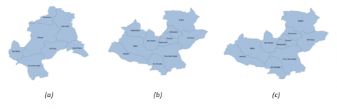
Currently, the department of Tlemcen has 53 municipalities, 20 daïras, and 07 health sectors. However, this was not always the case, because the administrative division of the department, with its different levels, has experienced many changes. To put in practice the proposed spatial interpolation method, we have chosen to restrict the scope of the discussed changes to those that have affected municipalities that are covered by the health sector which bears the same name as the department, the health sector of Tlemcen. Changes that have been taken into consideration have been grouped into three versions and are summarized in Figure 4.
Figure 4. Administrative division evolution at the municipality of Tlemcen
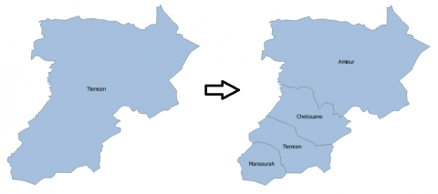
Figure 5. Evolution of the municipality of Tlemcen
The results we will discuss here concern calculating the weighting coefficients that are related to the lowest level of the spatial dimension, municipalities. By working with the three versions that emerged from the evolution of the studied municipalities, two transformation matrices must be defined: the first matrix allows us to move from version 1 to version 2, and the second one from version 2 to version 3.
3.3 Transformation matrices definition
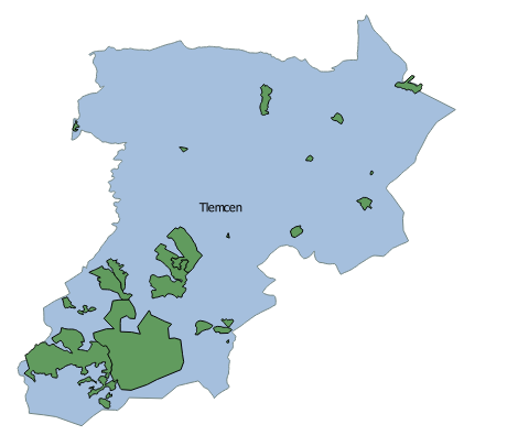
The transformation matrix to be defined between version 1 and version 2 concern the appearance of three new municipalities (Amieur, Chetouane, and Mansourah) inside the municipality of Tlemcen (see Figure 5). Based on Tlemcen municipality population, the agglomeration layer (see Figure 6), and the spatial interolation algorithm that was previously proposed, it is possible to produce the transformation matrix that must be defined between version 1 and version 2 (see Table 2.). Between version 2 and version 3, no weighting coefficient has to be calculated, because the only change that has taken place is related to the deletion of the municipality of Ouled Riah, since it is now covered by another health sector, therefore, each cell of the matrix of transformation contains either 0 or 1.
In this article, the proposed spatial interpolation method, which relies on the use of the population in calculating weighting coefficients, which in turn are used in estimating the number of people with tuberculosis in zones where the exact number is not known, can also be used in the estimation of indicators of other epidemics, and even indicators of public health since these indicators are primarily related to human presence in a given region.
Figure 6. Agglomerations belonging to the municipality of Tlemcen
In this article, we discussed the problem of spatial data warehouses evolution. Work on this theme culminated in the development of TUBERCOLAP, a SOLAP type multidimensional data exploration interface for tuberculosis surveillance. TUBERCOLAP is linked to a spatiotemporal data warehouse in which spatial and non-spatial dimensions can evolve. Our contribution differs from the others by the introduction of a spatial interpolation method based on the combined use of the map of agglomerations and the population of municipalities in estimating measure values to be assigned to zones when the exact values are not known.
Table 2. Transformation matrix defined between version 1 And version 2
|
Tlemcen |
Béni mester |
Ain Fezza |
Terny |
Amieur |
Chetouane |
Mansourah |
sabra |
Bouhlou |
Ain Ghoaba |
Ouled Riyah |
|
|
Tlemcen |
0.48 |
0 |
0 |
0 |
0.07 |
0.21 |
0.24 |
0 |
0 |
0 |
0 |
|
Beni mester |
0 |
1 |
0 |
0 |
0 |
0 |
0 |
0 |
0 |
0 |
0 |
|
Ain Fezza |
0 |
0 |
1 |
0 |
0 |
0 |
0 |
0 |
0 |
0 |
0 |
|
Terny |
0 |
0 |
0 |
1 |
0 |
0 |
0 |
0 |
0 |
0 |
0 |
|
Bensekrane |
0 |
0 |
0 |
0 |
0 |
0 |
0 |
0 |
0 |
0 |
0 |
|
Sidi Abdelli |
0 |
0 |
0 |
0 |
0 |
0 |
0 |
0 |
0 |
0 |
0 |
|
Ouled Mimoun |
0 |
0 |
0 |
0 |
0 |
0 |
0 |
0 |
0 |
0 |
0 |
We can use the spatial interpolation method as described in this article to estimate the value of any public health indicator when the exact value is not known. We can also improve the quality of the approximations made using this method, but in a more specific context, such as that of tuberculosis, by integrating other sources of data that are directly correlated with the values of the studied indicator (like humidity levels and the classification of each zone in urban or rural areas in the case of tuberculosis) in the form of thematic layers, so, instead of using the agglomeration layer only, we work with the map that results from the intersection of the agglomeration layer with the other layers.
[1] Eder J, Koncilia C, Morzy T. (2001). A model for a temporal data warehouse.
[2] Eder J, Koncilia C, Morzy, T. (2002). The COMET metamodel for temporal data warehouses. In International Conference on Advanced Information Systems Engineering. Springer, Berlin, Heidelberg 5: 83-99. http://dx.doi.org/10.1007/3-540-47961-9_9
[3] Morzy T, Wrembel R. (2004). On querying versions of multiversion data warehouse. In Proceedings of the 7th ACM International Workshop on Data Warehousing and OLAP ACM 11(12-13): 92-101. http://dx.doi.org/10.1145/1031763.1031781
[4] Wrembel R, Bębel B. (2005). Metadata management in a multiversion data warehouse. On the Move to Meaningful Internet Systems 2005: CoopIS, DOA, and ODBASE 3761: 1347-1364. http://dx.doi.org/10.1007/978-3-540-70664-9_5
[5] Tchounikine A, Miquel M, Laurini R, Ahmed TO, Bimonte S, Baillot V. (2005). Panorama de travaux autour de l'intégration de données spatio-temporelles dans les hypercubes. In EDA 6: 21-33.
[6] Plumejeaud, C. (2013). Modèles et méthodes pour l'information spatio-temporelle évolutive. Doctoral dissertation, Université Grenoble Alpes.
[7] Lam NSN. (1983). Spatial interpolation methods: a review. The American Cartographer 10(2): 129-150. http://dx.doi.org/10.1559/152304083783914958
[8] Wu SS, Qiu X, Wang L. (2005). Population estimation methods in GIS and remote sensing: A review. GIScience & Remote Sensing 42(1): 80-96. http://dx.doi.org/10.2747/1548-1603.42.1.80
[9] Briggs D, Fecht D, De Hoogh K. (2007). Census data issues for epidemiology and health risk assessment: experiences from the Small Area Health Statistics Unit. Journal of the Royal Statistical Society: Series A (Statistics in Society) 170(2): 355-378. http://dx.doi.org/10.1111/j.1467-985X.2006.00467.x
[10] Fisher PF, Langford M. (1996). Modeling sensitivity to accuracy in classified imagery: A study of areal interpolation by dasymetric mapping. The Professional Geographer 48(3): 299-309. http://dx.doi.org/10.1111/j.0033-0124.1996.00299.x