F. Ouagueni | M. Boumehraz | Belhamdi
OPEN ACCESS
The solid oxide fuel cell (SOFC) is broadly used for distributed and clean power generation. The main problem related to SOFC lies in the difficulties to control the output voltage of the SOFC due to the strong nonlinearity, the rapid changes of the load and the limited fuel flow. The objective of the control of the SOFC system is to maintain the output voltage at a constant level and the fuel utilization rate in a safety interval. In this context, a multiple-input multiple-output (MIMO) discrete-time Takagi-Sugeno (TS) fuzzy dynamic model with feed forward input is used in this paper to describe the dynamic properties of the nonlinear voltage and the fuel utilization rate in a tubular SOFC system. This obtained fuzzy model will be used for the application of constrained fuzzy model predictive control. The simulation results are provided to show the accuracy and the effectiveness of the proposed strategy.
solid oxide fuel cell (SOFC), nonlinear system’s modeling, Takagi-Sugeno (TS) fuzzy model, model predictive control
The solid oxide fuel cell (SOFC) is a full of promise technology to produce electrical energy. It allows us to directly convert chemical energy into electrical energy and heat. The SOFC has evoked a substantial attentiveness because it provides broad application ranges, a fuel choice’s flexibility, a high system efficiency and the feasibility of operation with an internal reformer. When we use a solid-state ceramic electrolyte, SOFCs are characterized by high temperature range (i.e., 600°C-1000°C). This temperature is easier to maintain due to the lack of cell corrosion [1].
Among the factors affecting over the life of the SOFC is the significant change in fuel utilization due to transients in the load. Therefore, the fuel utilization rate $U_{f}$ is considered among of the most important control variables of the SOFC system. For protecting the SOFC, $U_{f}$ must be in the desired range is from $70 \%$ to $90 \%$ with an optimal operating point about $80 \%$. since a $U_{f}<70 \%$ where a very important part of the fuel is underused, that leads to the decrease in the economic efficiency of SOFC, otherwise, a $U_{f}>90 \%$ may lead to a permanent damage risk to the cells as a result of fuel starvation.
Fuel cells’ analysis can be categorized into two types of modeling, dynamic modeling and steady state modeling. In references [2, 3], the nonlinear dynamics’ SOFC modeling has been investigated. Great efforts, on SOFC modeling, have been made by many researchers in the sake of improving its performance [4, 5].
The most common method to study a system with a nonlinear model is to approximate it by a single linear model (linearization around an equilibrium point). The linear model can be just seen as a local description of the system, which is considered as a drawback of this approach. A comprehensive approach based on the use of several models around different operating points has been developed in recent years. The interpolation of these local models through standard activation functions allows to modeling the nonlinear global system [6, 7]. This approach is based on using Takagi–Sugeno (TS) fuzzy models [8], known for their universal approximation property.
In control community, for its capability to represent nonlinear dynamics, fuzzy dynamic models of the TS type is broadly accepted [8-10]. Fuzzy modeling and identification from measured data are considered as efficient tools to approximate uncertain nonlinear systems. Since the TS model needs less rules compared to the other models, it has attracted a huge attention from researchers. This model has simple fuzzy implication and each rule’s consequence with linear function can describe the input–output mapping in a large range [11]. The TS Fuzzy Modeling of SOFC System has been widely used in several papers [12-14].
For multivariable industrial processes with slow dynamics, the model predictive control (MPC) is known as a powerful control approach which made it a hot research topic during last three decades. MPC is able to control multivariable systems under various constraints in an optimal way [12]. The control actions are to be computed by solving a receding-horizon optimization problem at each sampling time instant, for MPC while only the predetermined control law is used in conventional optimal control. The linear control plant models are the basic formulations of the MPC algorithms. These latter can be formulated as easy to solve, linear–quadratic optimization problems. Nevertheless, the application of these algorithms to a nonlinear plant may bring unworthy results, and it may generally lead to a non–convex optimization problem that is a hard-to-solve and a computationally-demanding problem. In practice, we use suboptimal algorithms that consist of approximating the nonlinear model at each algorithm’s iteration. At each algorithm’s iteration, the standard linear–quadratic optimization problem is formulated and solved where various kinds of nonlinear models can be adopted. The TS fuzzy model is one of the most efficient nonlinear models [11, 12, 14].
When the load changes, the output voltage of the SOFC system and the fuel utilization rate can not be kept constant. To guarantee that the fuel utilization operates within a safe range, two control strategies can be considered. The first one consists of maintaining a constant output voltage at the SOFC. In the second strategy, we have to directly control the input hydrogen fuel in proportion to the stack current, so we can achieve a constant utilization control. When the load changes, to guarantee the fuel utilization within a desired safe range, one proper value for output voltage can be used [11].
To control the SOFC system, there exist many different methods. The model predictive control (MPC) which is the widely used one, was considered in [15, 16]. In this paper, we have proposed a control strategy that consists of a predictive control based on a nonlinear auto-regressive model with exogenous input (NARX) fuzzy dynamic model. In addition to maintaining the fuel utilization within a safe range, our model is capable of preventing the electrolyte’s damage by maintaining the pressure difference, which consists of the difference between the partial pressures of the hydrogen/oxygen in the anode and the cathode compartments of the fuel cell, below 8KPa under transient conditions and 4 KPa under normal operation [17]. The hydrogen/oxygen ratio $r_{H_{-} O}$, which consists of the inlet hydrogen flow over inlet oxygen flow, is also considered in the proposed control strategy. In this latter, it is better to keep the hydrogen/oxygen ratio around 1.145, as in [17].
In this paper, we will use the dynamic model of the SOFC type fuel cell proposed in [18], to form a combined two MISO (multiple-input single-output) discrete-time TS fuzzy dynamic models with linear consequents, one for the output voltage and another for the fuel utilization. This model facilitates the control of the SOFC system. After that, we have proposed a control strategy that consists of a predictive control based on the aforementioned model. The rest of this paper is structured as follows. In section 2, we will briefly describe the SOFC dynamic model. The multi-variable NARX TS fuzzy model will be presented in section 3. In section 4, we will discuss the constrained fuzzy predictive control. After that, in section 5, the simulation results will be provided and discussed. Finally, we will conclude the paper.
Using electrochemical reactions, the chemical energy in Hydrogen (H2) and Oxygen (O2) can be directly converted into electrical energy by fuel cells. So far, tubular SOFC dynamic model has been broadly investigated. Thus we’ll concisely review this model based on previous researches [3-4, 18].
Figure 1. Schematic diagram of a SOFC
The anode and cathode channels are the basic components of the SOFC system. In the fuel cell, we supply the fuel to the anode and the air to the cathode. At the cathode, oxygen molecules accept electrons from the external circuit and change to oxygen ions. At the anode, water will be produced when the negative ions go across the electrolyte and combine with the hydrogen. Within the cell, the following electrochemical reactions occur
Anode reaction:
$H_{2}+O^{2} \rightarrow H_{2} O+2 e^{-}$ (1)
Cathode reaction:
$1 / 2 O_{2}+2 e^{-} \rightarrow O^{-2}$ (2)
Total reaction:
$H_{2}+1 / 2 O_{2} \rightarrow H_{2} O$ (3)
The output voltage is the most important variable in the SOFC system because most of control intention is to make the actual voltage trajectory and the desired voltage trajectory the same. Based on the dynamic SOFC system and under Matlab/Simulink environment, we’ve developed a simulation model for the SOFC system. This latter is based on [18] as regards to the expression for the partial pressures of hydrogen, oxygen and water. To calculate the fuel cell output voltage, we will use the expressions for partial pressures. The partial pressures inside the channel of hydrogen, oxygen and water can be written in the Laplace transform domain as follows [18]:
$P_{H_{2}}(s)=\frac{1}{\left(1+\tau_{a} s\right)}\left[q_{H}^{i n}(s)+\tau_{a} P_{H_{2}}(0)-\frac{P_{a}}{4 F M_{a}} I(s)\right]$ (4)
$P_{O_{2}}(s)=\frac{1}{\left(1+\tau_{c} s\right)}\left[q_{O}^{i n}(s)+\tau_{c} P_{O_{2}}(0)-\frac{P_{c}}{4 F M_{c}} I(s)\right]$ (5)
$P_{H_{2} O}(s)=\frac{1}{\left(1+\tau_{a} s\right)}\left[q_{H_{2} O}(s)+\tau_{a} P_{H_{2} O}(0)+\frac{P_{a}}{4 F M_{a}} I(s)\right]$ (6)
where $q_{O}^{i n}$ and $q_{H}^{i n}$ are the molar flows of oxygen and hydrogen at the input of the stack, $\tau_{a}=V_{a} P_{a} / 2 M_{a} R T$ and $\tau_{c}=V_{c} P_{c} / 2 M_{c} R T$ are the time constant (second) for the hydrogen and oxygen flows. The physical meaning of $\tau_{a},$ is that it will take $\tau_{a}$ seconds to fill a tank of volume $V_{a} / 2$ at pressure $P_{a}$ if the mass flow rate is $M_{a} .$ The same physical meaning for $\tau_{c}$ [18].
Several types of irreversible losses, such as activation, concentration and ohmic losses will decrease the actual cell potential from its ideal potential. The following are the polarization equations [19]
$V_{a c t}=\partial+\beta \log I$ (7)
$V_{c o n c}=\frac{R T}{n F} \ln \left(1-\frac{I}{I_{l}}\right)$ (8)
$V_{o h m}=I r$ (9)
We can write the cell resistance r as
$r=r_{0} \exp \left[\alpha\left(\frac{1}{T_{0}}-\frac{1}{T_{s}}\right)\right]$ (10)
where $r_{0}$ is the internal resistance at temperature $T_{0}$ and $\alpha$ is a constant.
Considering an ideal behavior and a constant temperature, the SOFC output voltage $V_{S}$ is given by
$V_{s}=E-V_{a c t}-V_{o j m}-V_{c o n c}$ (11)
E , is the SOFC open-circuit voltage, which can be written as
$E=N_{\text {cell}}\left(E_{0}+\frac{R T}{4 F} \ln \left[\frac{\left(P_{H_{2}}\right)^{2} \cdot P_{O_{2}}}{P_{H_{2} O}}\right]\right)$ (12)
where $N_{c e l l}$ is the number of series-connected cells and $E_{0}$ is the standard reference potential state, $298 \mathrm{k}$ and 1 atm pressure.
The fuel utilization factor $U_{f}$ is the important performance index for a SOFC, defined as the ratio between the consumed hydrogen flow in reaction $q_{H}^{r}$ and the inlet hydrogen flow $q_{H}^{i n}$ that is:
$U_{f}=\frac{q_{H}^{r}}{q_{H}^{i m}}$ (13)
The inlet hydrogen flow can be controlled so that the fuel utilization factor will be regulated at an optimal value about 80% [20].
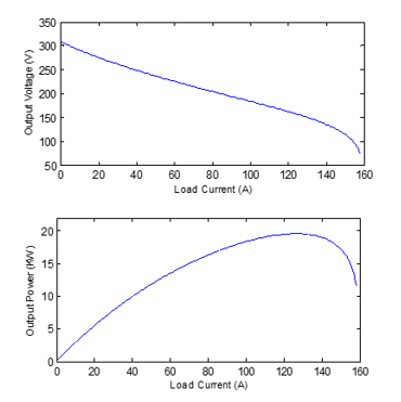
Figure 2. Voltage/power-load current characteristics of SOFC in open-loop
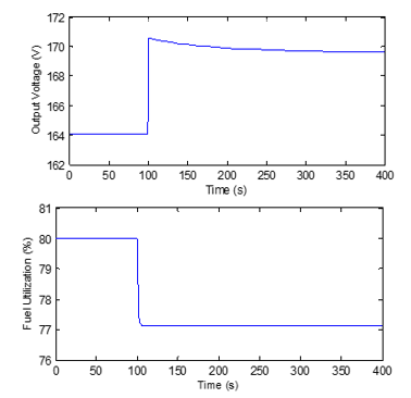
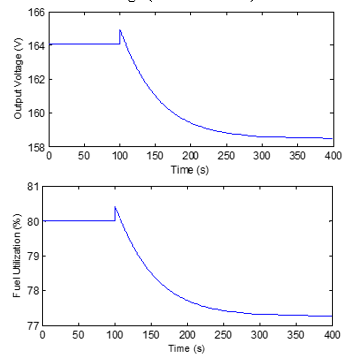
The voltage/power-load current characteristics of the SOFC in open loop are depicted in Figure 2, which shows the nonlinear behavior of SOFC in an extended operating regime. Furthermore, the dynamic responses in open loop of the SOFC system to stepwise changes of inputs $q_{H}^{i n}, q_{O}^{i n},$ and $I_{L}$ are given in Figure 3–5, respectively.
One can define the ratio between inlet hydrogen flow and oxygen flow as [20]
$r_{H_{-} O}=\frac{q_{H}^{m}}{q_{o}^{m}}$ (14)
In the fuel cell anode and cathode compartments, the difference in the partial pressures of hydrogen and oxygen, $\Delta P$ is given by
$\Delta P=P_{H_{2}}-P_{O_{2}}$ (15)
Figure 3. SOFC system step response to load current change (-5A)
Figure 4. SOFC system step response to hydrogen flow rate change (+0.4×10⁻²mol/s)
Figure 5. SOFC system step response to oxygen flow rate change (+0.4×10⁻²mol/s)
According to [20], for safety reasons, the value of this ratio is chosen such that the difference between the pressure of hydrogen and that of oxygen must not exceed 4 kPa under normal operating conditions and 8 KPa under transient conditions.
3.1 NARX model structure
Consider a general multiple-input multiple-output (MIMO) nonlinear system with $m$ inputs: $u \in U \subset \Re^{m}$, and $p$ outputs: $y \in Y \subset \Re^{P}$. This system is approximated by a collection of coupled MISO discrete-time TS fuzzy dynamic models of the input-output NARX type [21]
$\mathrm{y}_{1}(k+1)=R_{l}\left(\varphi_{l}(k), \mathrm{u}(k)\right), \quad l=1,2, \ldots, p$ (16)
where, $u(k) \in \mathscr{I}^{m}$ is the input vector containing the current inputs, and $\varphi_{l}(k) \in \mathscr{I}^{q}$ is the regression vector which includes current and lagged outputs and inputs:
$\varphi_{I}(k)=\left[\mathrm{y}_{1}(k), \ldots, \mathrm{y}_{p}(k), \mathrm{u}_{1}(k-1), \ldots, \mathrm{u}_{m}(k-1)\right]^{T}$ (17)
with
$y_{i}(k)=\left[y_{i}(k), y_{i}(k-1), \ldots, y_{i}\left(k-n_{y, i}\right)\right], i=1, \ldots, p$ (18)
$u_{j}(k-1)=\left[u_{j}(k-1), u_{j}(k-2), \ldots, u_{j}\left(k-n_{u, j}\right)\right], j=1, \ldots, m$ (19)
where, $n_{y, i}$ is the number of lagged values for the $i^{\text {th }}$ output, and $n_{u, j}$ is the number of lagged values for the $j^{\text {th }}$ input.
In the following equation, $l$ fuzzy rules are used to describe the TS MISO fuzzy model as in [8]
$R_{l i}:$ if $\varphi_{l 1}(k)$ is $M_{l l, 1}$ and $\ldots$ and $\varphi_{l q}(k)$
is $\mathrm{M}_{\text {Ii, } q}$ and $u_{1}(k)$ is $\mathrm{M}_{l_{l}, q+1}$ and $\ldots$ and $u_{m}(k)$ is $\mathrm{M}_{l l, q+m}$ then
$y_{l_{l}}(k+1)=\lambda_{l_{i}} \varphi_{l}(k)+\sigma_{l_{l}} \mathbf{u}(\mathbf{k})+\eta_{i_{i}}$
$i=1,2, \dots$
$r_{l} \quad l=1,2, \dots, L$ (20)
where, $R_{l}$ denotes the $l$ th fuzzy inference rule, $L$ the number of inference rules, $\varphi_{l}(k)$ the premise measurable variables, $r_{l}$ is the number of rules for the $l^{\text {th }}$ output, $\lambda_{l i}$ and $\sigma_{l i}$ are vectors containing the consequent parameters, $M_{l i}$ are the antecedent fuzzy sets of the $i$ th rule and $\eta_{l i}$ is the offset.
The weighted average of the linear consequents in the individual rules are used to compute the model output as follows [21]
$y_{l}(k+1)=\frac{\sum_{i=1}^{r_{i}} \omega_{l i}\left(\lambda_{i i} \varphi_{l}(k)+\sigma_{h i} \mathrm{u}(\mathrm{k})+\eta_{i j}\right)}{\sum_{i=1}^{n} \omega_{l i}}$ (21)
The product of the membership degrees of the antecedent variables (states and inputs) in the $i^{\text {th }}$ rule $\omega_{l i}$ is its degree of fulfillment.
3.2 Parameter identification of the NARX model
After determining the NARX model structure, the least squares algorithm can be used to estimate the parameters of the NARX model as follows
$\hat{\theta}=\left[Q^{T} Q\right]^{-1} Q^{T} \mathrm{Y}$ (22)
where, $\hat{\theta}=\left[\hat{a}_{1}, \hat{a}_{1}, \ldots, \hat{a}_{n_{y, i}}, \hat{b}_{1}, \hat{b}_{1}, \ldots, \hat{b}_{n_{u, j}}\right]^{T}$ is the estimated parameters of the NARX model and
$Q=[\mu(1), \mu(2), \ldots, \mu(N-1)]^{T}$ (23)
$Y=[y(1), y(2), \ldots, y(N)]^{T}$ (24)
In this work, the basic global model for calculating the prediction is a discret TS fuzzy dynamic model with feedforward input given by
$\left\{\begin{array}{ll}x(k+1)=A_{h} x(k)+B_{h} u(k)+B_{f_{h}} u_{f}(k) & l=1, \ldots, L \\ y(k)=C_{h} x(k) & \end{array}\right.$ (25)
where,
$\begin{aligned} A_{\hbar}=\sum_{l=1}^{L} h_{l} A_{l}, & B_{h}=\sum_{l=1}^{L} h_{l} B_{l}, \quad B_{f i}=\sum_{l=1}^{L} h_{l} B_{f l} \\ & C_{h}=\sum_{l=1}^{L} h_{l} C_{l} \\ & h=h_{1}, \ldots, h_{L} \end{aligned}$ (26)
where, $x(k) \in \Re^{n}$ is the system state variables, $u_{f}(k) \in \Re^{m_{f}}$ and $u(k) \in \mathscr{R}^{m}$ are respectively the feedforward and manipulated inputs, $y(k) \in \mathscr{R}^{p}$ the outputs variables and $\left(A_{l}, B_{l}, B_{f_{l}}, C_{l}\right)$ is the $l^{th}$ local model, which is subject to the constraints in the control $u(k)$
The augmented model can be obtained [15]
$\mathrm{x}(k+1)=\mathrm{Ax}(k)+\mathrm{B} \Delta u(k)+\mathrm{B}_{f} \Delta u_{f}(k)$
$\mathrm{y}(k)=\mathrm{Cx}(k)$ (27)
where,
$\mathrm{x}(k)=\left[\begin{array}{c}\Delta \mathrm{r}(k) \\ y(k)\end{array}\right], \mathrm{A}=\left[\begin{array}{cc}A_{n} & O \\ C_{h} A_{n} & I\end{array}\right], \mathrm{B}=\left[\begin{array}{c}B_{n} \\ C_{n} B_{n}\end{array}\right], \mathrm{B}_{f}=\left[\begin{array}{c}B_{f_{n}} \\ C_{h} B_{f_{h}}\end{array}\right], \mathrm{C}=\left[\begin{array}{ll}I & I\end{array}\right]$
$\Delta x(k)=x(k)-x(k-1), \Delta u(k)=u(k)-u(k-1)$
$\Delta u_{f}(k)=u_{f}(k)-u_{f}(k-1)$ (28)
The cost function I to be minimized at each sampling period penalizes the deviations of the predicted outputs $\hat{y}(k+j | k)$ of a reference trajectory $y_{r}(k+j | k)$ and the variations of the control vector $\Delta u(k),$ it is usually given by
$\min _{u} \mathfrak{T}=\left\|Y_{r}-\hat{Y}\right\|_{S}^{2}+\|\Delta \mathrm{U}\|_{R}^{2}$
subject to $\underline{u} \leq u \leq \bar{u}$
$\Delta u \leq \Delta u \leq \overline{\Delta u}$ (29)
where, $S$ and $R$ are the weighting matrices, the prediction model based on the fuzzy model (25), can be got as
$\hat{Y}=\Theta \mathrm{x}(k)+\Gamma \Delta \mathrm{U}+\Gamma_{f} \Delta u_{f}(k)$
$\hat{Y}=\left[y(k+1 | k) y(k+2 | k) \ldots y\left(k+H_{p} | k\right)\right]^{T}$
$\Delta \mathrm{U}=\left[\Delta u(k+1 | k) \Delta u(k+2 | k) \ldots \Delta u\left(k+H_{c} | k\right)\right]^{T}$
$\Delta u_{f}=\left[\Delta u_{f}(k+1 | k) \Delta u_{f}(k+2 | k) \ldots \Delta u_{f}\left(k+H_{c} | k\right)\right]^{T}$ (30)
$\Theta=\left[\begin{array}{c}\mathrm{CA} \\ \mathrm{CA}^{2} \\ \vdots \\ \mathrm{CA}^{H_{p}-1} \\ \mathrm{CA}^{H_{p}}\end{array}\right], \Gamma=\left[\begin{array}{cccc}\mathrm{CB} & 0 & \cdots & 0 \\ \mathrm{CAB} & \mathrm{CB} & \cdots & 0 \\ \vdots & \vdots & \ddots & \vdots \\ \mathrm{CA}^{H_{p}-2} \mathrm{B} & \mathrm{CA}^{H_{p}-3} \mathrm{B} & \cdots & \mathrm{CA}^{H_{p}-H_{c}-1} \mathrm{B} \\ \mathrm{CA}^{H_{p}-1} \mathrm{B} & \mathrm{CA}^{H_{p}-2} \mathrm{B} & \cdots & \mathrm{CA}^{H_{p}-H_{c}}\end{array}\right]$ $\Gamma_{f}=\left[\begin{array}{c}\mathrm{CB}_{f} \\ \mathrm{CAB}_{f} \\ \vdots \\ \mathrm{CA}^{H_{p}-1} \mathrm{B}_{f} \\ \mathrm{CA}^{H_{p}-2} \mathrm{B}_{f}\end{array}\right]$ (31)
The parameter $H_{p}$ represents the maximum prediction horizon and $H_{c}$ represents the control horizon.
The constraints of the manipulated variables can be expressed in the following matrix form
$\underline{U} \leq Q \Delta \mathrm{U} \leq \bar{U} \Rightarrow\left[\begin{array}{c}Q \\ -Q\end{array}\right] \Delta U \leq\left[\begin{array}{c}\bar{U} \\ -\underline{U}\end{array}\right]$ (32)
where
$\underline{U}=[\underline{u}-u(k-1), \ldots, \underline{u}-u(k-1)]_{1 \times\left(n_{u} H_{c}\right)}^{T}$
$\underline{\Delta U}=[\underline{\Delta u}, \ldots, \underline{\Delta u}]_{1 \times\left(n_{u} H_{c}\right)}^{T}$
$\bar{U}=[\bar{u}-u(k-1), \ldots, \bar{u}-u(k-1)]_{1 \times\left(n_{u} H_{c}\right)}^{T}$
$\overline{\Delta U}=[\overline{\Delta u}, \ldots, \overline{\Delta u}]_{1 \times\left(n_{u} H_{c}\right)}^{T}$
$Q=\left[\begin{array}{cccc}I & & & \\ I & I & & \\ \vdots & \vdots & \ddots & \\ I & I & \cdots & I\end{array}\right]_{H_{c} \times H_{c}}$ (33)
where $I$ is an identity matrix of dimension $n_{u} \times n_{u}$ and $n_{u}$ is the number of manipulated variables.
Then the cost function (29) can be rewritten as follows
$\begin{align} & \underset{u}{\mathop{\min }}\,\Im =\left\| {{Y}_{r}}-\Theta \text{x(}k\text{)}-\Gamma \Delta \text{U}-{{\Gamma }_{f}}\Delta {{u}_{f}}(k) \right\|_{S}^{2}+\left\| \Delta \text{U} \right\|_{R}^{2} \\ & subject\,to\,\,\,\,\left[ \begin{matrix} Q \\ -Q \\\end{matrix} \right]\Delta U\le \left[ \begin{matrix} \overline{U} \\ -\underline{U} \\\end{matrix} \right] \\ & \,\,\,\,\,\,\,\,\,\,\,\,\,\,\,\,\,\,\,\,\,\,\,\,\,\,\,\underline{\Delta U}\,\le \Delta U\le \,\overline{\Delta U}\,\,\,\,\,\,\,\,\,\,\,\,\,\,\,\,\,\,\,\,\,\,\,\,\,\,\,\,\,\,\, \\\end{align}$ (34)
5.1 TS fuzzy dynamic model identification of SOFC System
According to section 3, we can identify two combined MISO discrete-time TS fuzzy dynamic models of the Tubular SOFC System, one for the output voltage and another for the fuel utilization rate. In our work, each TS model has three inputs:
(1) Two manipulated inputs: the fuel flow $q_{H}^{i n}$ and the oxygen flow $q_{O}^{i n}$.
(2) One feedforward input: load current $I_{L}$.
For the premise variable $I_{L}$, we choose the membership function as
$"Low": M F^{1}=\left\{\begin{array}{ll}1, & \text { if } I_{L} \leq 80 \\ 1-\frac{I_{L}-80}{100-80}, & \text { if } 80 \leq I_{L} \leq 100 \\ 0, & \text { if } I_{L} \geq 100\end{array}\right.$ (35)
$"Middle": M F^{2}=\left\{\begin{array}{ll}1-\mathrm{MF}^{1} & \text { if } \quad I_{L} \leq 100 \\ 1-\mathrm{MF}^{3} & \text { if } \quad I_{L} \geq 120\end{array}\right.$ (36)
$"$ High": $M F^{1}=\left\{\begin{array}{ll}0, & \text { if } I_{L} \leq 100 \\ \frac{I_{L}-100}{120-100}, & \text { if } 100 \leq I_{L} \leq 120 \\ 1, & \text { if } I_{L} \geq 120\end{array}\right.$ (37)
The membership functions are shown in figure 6.
Figure 6. Membership function of load current IL in fuzzy SOFC model
and by utilizing the method described in section 3, with the two following regression vectors, which represent the first MISO model and the second MISO model respectively.
$\varphi_{1}(k)=\left[V_{s}(k), V_{s}(k-1), V_{s}(k-2), q_{H}^{i n}(k)\right.$
$q_{H}^{i n}(k-1), q_{H}^{i n}(k-2), q_{0}^{i n}(k), q_{o}^{i n}(k-1)$
$\left.q_{0}^{i n}(k-2), I_{L}(k), I_{L}(k-1), I_{L}(k-2)\right]^{T}$ (38)
$\varphi_{2}(k)=\left[U_{f}(k), U_{f}(k-1), U_{f}(k-2), q_{H}^{i n}(k),\right.$
$q_{H}^{i n}(k-1), q_{H}^{i n}(k-2), q_{O}^{i n}(k), q_{o}^{i n}(k-1)$
$\left.q_{o}^{i n}(k-2), I_{L}(k), I_{L}(k-1), I_{L}(k-2)\right]^{T}$ (39)
The two TS fuzzy dynamic models of the SOFC system can be easily identified, as follows
(1) The 1st MISO TS fuzzy model
Rule1:IF current load $I_{L}$ is Low, THEN
$V_{s}(k+1)=1.15778 V_{s}(k)+0.55134 V_{s}(k-1)-0.70898 V_{s}(k-2)$
$+0.35258 q_{H}^{i n}(k)-0.42206 q_{H}^{i n}(k-1)+0.34322 q_{H}^{i n}(k-2)$
$-0.39029 q_{0}^{i n}(k)-0.86401 q_{0}^{i n}(k-1)-0.49042 q_{0}^{i n}(k-2)$
$-0.04630 I_{L}(k)+0.01094 I_{L}(k-1)+0.03489 I_{L}(k-2)$
Rule2: IF current load $I_{L}$ is Middle, THEN
$V_{s}(k+1)=0.54731 V_{s}(k)+0.61559 V_{s}(k-1)-0.21283 V_{s}(k-2)$
$-0.98644 q_{H}^{i n}(k)+0.20439 q_{H}^{i n}(k-1)-0.22678 q_{H}^{i n}(k-2)$
$+0.83198 q_{0}^{i n}(k)-0.99770 q_{0}^{i n}(k-1)-0.07510 q_{0}^{i n}(k-2)$
$+0.03764 I_{L}(k)-0.02100 I_{L}(k-1)+0.01478 I_{L}(k-2)$
Rule3: IF current load $I_{L}$ is $\mathrm{High}$, THEN
$V_{s}(k+1)=1.04761 V_{s}(k)+0.69987 V_{s}(k-1)-0.74506 V_{s}(k-2)$
$-0.92862 q_{H}^{i n}(k)-0.64784 q_{H}^{i n}(k-1)+0.44326 q_{H}^{i n}(k-2)$
$-0.05303 q_{0}^{i n}(k)-0.69455 q_{0}^{i n}(k-1)-0.31775 q_{0}^{i n}(k-2)$
$-0.04519 I_{L}(k)+00618 I_{L}(k-1)+0.03769 I_{L}(k-2)$ (40)
(2) The 2nd MISO TS fuzzy model
Rule1 : IF current load $I_{L}$ is Low,THEN
$U_{f}(k+1)=0.0844 U_{f}(k)+0.1577 U_{f}(k-1)-0.0590 U_{f}(k-2)$
$-0.5880 q_{H}^{i n}(k)+0.8959 q_{H}^{i n}(k-1)-0.8359 q_{H}^{i n}(k-2)$
$-0.7886 q_{0}^{i n}(k)-0.7159 q_{0}^{i n}(k-1)-0.6671 q_{0}^{i n}(k-2)$
$+0.0172 I_{L}(k)+0.0074 I_{L}(k-1)-0.0218 I_{L}(k-2)$
Rule2: IF current load $I_{L}$ is Middle , THEN
$U_{f}(k+1)=0.8624 U_{f}(k)+0.4573 U_{f}(k-1)+0.4757 U_{f}(k-2)$
$-0.8732 q_{H}^{i n}(k)+0.7209 q_{H}^{i n}(k-1)+0.8688 q_{H}^{i n}(k-2)$
$+0.9688 q_{o}^{i n}(k)+0.7179 q_{0}^{i n}(k-1)+0.5711 q_{o}^{i n}(k-2)$
$+0.0268 I_{L}(k)-0.6448 I_{L}(k-1)-0.2028 I_{L}(k-2)$
Rule3: IF current load $I_{L}$ is $\mathrm{High}$, THEN
$U_{f}(k+1)=-0.7321 U_{f}(k)-0.9382 U_{f}(k-1)+0.8783 U_{f}(k-2)$
$-0.3974 q_{H}^{i n}(k)-0.4089 q_{H}^{i n}(k-1)-0.3341 q_{H}^{i n}(k-2)$
$-0.0659 q_{0}^{i n}(k)+0.2964 q_{0}^{i n}(k-1)-0.9495 q_{0}^{i n}(k-2)$
$+0.6844 I_{L}(k)+0.1181 I_{L}(k-1)+0.7082 I_{L}(k-2)$ (41)
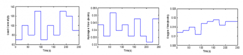
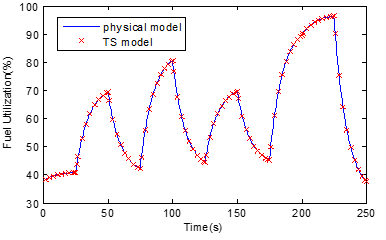
The results in figure 7-9 respectively represent the input signals of the SOFC system, the output voltage and the fuel utilization rate of the SOFC system, and those of the TS fuzzy models.
To evaluate the modeling results, the root mean square error (RMSE) defined in the following equation is considered.
$R M S E=\sqrt{\frac{1}{N} \sum_{k=1}^{N}(y(k)-\hat{y}(k))^{2}}$ (42)
where, $N$ is the number of sample data considered for modeling, $\hat{y}(k)$ is the fuzzy system output and $y(k)$ is the actual output.
The RMSE of the output voltage and the fuel utilization are 0.1436 and 0.1328 respectively. These values are compared in table 1, with the results obtained for other modeling methods. One can conclude that, using the proposed TS fuzzy models, the dynamic behavior of the physical SOFC model can be approximated with good accuracy.
Figure 7. Excitation input signals to SOFC system
Figure 8. Dynamic output of SOFC voltage
Figure 9. Fuel utilization response
Table 1. Comparison of modeling methods
|
References |
Identified models |
RMSE |
|
|
Vs |
Uf |
||
|
[11] |
GA-RBF (Genetic Algorithm-Radial Basis function) neural network model |
1.1836 |
- |
|
[19] |
NARMA (Nonlinear Autoregressive-moving Average) TS fuzzy model |
0.2582 |
- |
|
[22] |
Modified OIF (Output–Input Feedback) Elman neural network model |
0.2573 |
- |
|
This paper |
NARX TS fuzzy |
0.1436 |
0.1328 |
5.2 Fuzzy predictive control of a tubular SOFC System
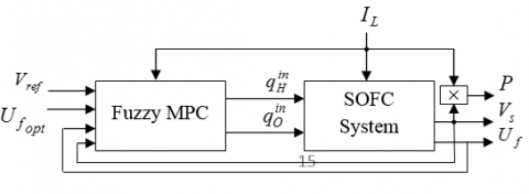
As we mentioned earlier, the power generation in the SOFC power plant is directly affected by the change in the external load. In fact, for stable operation of electrical equipment, the output voltage of this power system must be at a required constant value. To achieve this objective, we integrate a controller into the SOFC system. In this work, we use the proposed Fuzzy Model Feed forward Predictive Control (FMFPC) method detailed in section 4 and shown in figure 10
Figure 10. Diagram of the proposed FMFPC
Following the same steps as in [12], we can rewrite the fuzzy models in equations (40) and (41) as a state space model with feed forward input defined in $(25),$ where $u(k)$ is a manipulated input vector composed of hydrogen flow rate and oxygen flow rate, $u_{f}(k)$ is the feed forward input vector that consists of the load current, and $y(k)$ is an output vector composed of the output voltage and the fuel utilization rate.
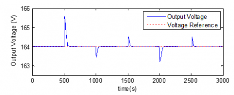
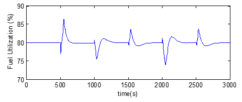
In this section, the FMFPC is used to control a SOFC given an output voltage equal to $164 \mathrm{V},$ a fuel utilization rate within a range is from $70 \%$ to $90 \%$ with an optimal operating point about $80 \%,$ and we respect the variation of $\Delta P$ and $r_{H_{-} O}$ in the previously mentioned margins. The FMFPC method used here is based on the Fuzzy Models in (25). The MPC parameters are chosen as: $H_{c}=3, H_{p}=10, Q=12 I$ and $R=0.4 I$.
In standard functioning, the load’s current of the SOFC system is 120 A. The voltage reference is assumed to be fixed at 164 V. To check the performance of the SOFC system we change the load’s current by a step of 500 seconds in a range of 90 to 130A (see figure 11). The proposed FMFPC is considered here. As can be seen from figure 12-14, when the load current fluctuates, the output voltage changes rapidly then returns back to the reference value, the fuel utilization rate remains in the required range and the monitored variables changes are kept within the safety range, so the proposed FMFPC can be used to maintain the output voltage in its reference value with guaranteed all the performances of SOFC considered before.
Figure 11. Load current variation
Figure 12. Trajectories of SOFC voltage by FMFPC
Figure 13. Fuel utilization response by FMFPC
Regarding the comparison with the results of $[15],$ the fuel/hydrogen flow rate and oxygen flow in [15] are fixed to be $r_{H_{-} O}=1.145,$ so their control system has only one active manipulated variable and slow load following response (around 200s). While in this paper, there are two independent control inputs $q_{H}^{\text {in }}$ and $q_{O}^{\text {in }}$ in data-driven control system and load following response less than 100 s, in general, more control freedom offers more opportunities for performance improvement. In this paper, we have taken into account the control performance in controller design and synthesis, so our proposed fuzzy predictive control system can maintain the load following ability with negligible tracking error.
Figure 14. Curves of monitoring performances
Figure 15. Curves of manipulated variables
In this work, we have developed a NARX MIMO constrained fuzzy predictive control strategy issued from a data-driven identification, in the aim of improving the load tracking performance of a SOFC system. This strategy guarantees a constant output voltage, a fuel utilization rate that operates in a safe range, a pressure difference below the required values and a hydrogen/oxygen ratio around 1.145. The simulation results show the accuracy of the proposed SOFC control strategy.
Parameters in the SOFC dynamic model [1]
$T=1173(K)$ Gas temperature
$R=8.3143(J /(\text {mol. } K))$ Gas constant
$F=96487(C / m o l)$ Faraday's constant
$P_{a}=P_{c}=3(a t m)$ Anode and cathode pressures
$V_{a}=61.7138 \times 10^{-6}\left(m^{3}\right)$ Volume of anode channel
$V_{c}=99.02 \times 10^{-6}\left(\mathrm{m}^{3}\right)$ Volume of cathode channel
$E^{0}=1.18(V)$ Standard reference potential
[1] Wang, Y., Yoshib, F., Watanabe, T., Weng, S. (2007). Numerical analysis of electrochemical characteristics and heat/ species transport for planar porous-electrode-supported SOFC. Journal of Power Source, 170(1): 101-110. https://doi.org/10.1016/j.jpowsour.2007.04.004
[2] Lee, T.H., Park, J.H., Lee, S.M., Lee, S.C. (2010). Nonlinear Model Predictive Control for Solid Oxide Fuel Cell System Based on Wiener Model. International Journal of Computer, Electrical, Automation, Control and Information Engineering, 4: 1935-1940.
[3] Marra, D., Pianese, C., Polverino, P., Sorrentino, M. (2016). Models for Solid Oxide Fuel Cell Systems: Exploitation of Models Hierarchy for Industrial Design of Control and Diagnosis Strategies. Springer-Verlag.
[4] Spivey, B.J., Edgar, T.F. (2012). Dynamic modeling, Simulation, and MIMO Predictive Control of a Tubular Solid Oxide Fuel Cell. Journal of Process Control, 22(8): 1502-1520. https://doi.org/10.1016/j.jprocont.2012.01.015
[5] Barelli, L., Bidini, G., Ottaviano, A. (2016). Solid Oxide Fuel Cell Modelling: Electrochemical Performance and Thermal Management During Load-Following Operation. Science Direct. Energy, 115: 107-219. https://doi.org/10.1016/j.energy.2016.08.107
[6] Gangulu, P., Kalam, A., Zayegh, A. (2017). Optimum Fuzzy Logic Control System Design using Cuckoo Search Algorithm for Pitch Control of a Wind Turbine. AMSE Journals, Advances C, 72(4): 266-280.
[7] Belhamdi, S., Goléa, A. (2013). Fuzzy logic Control of Asynchronous Machine Presenting Defective Rotor Bars. AMSE Journals, Advances C, 68(2): 54-63.
[8] Takagi, T., Sugeno, M. (1985). Fuzzy Identification of Systems and Its Applications to Modeling and Control. IEEE Transactions on Systems Man and Cybernetics, 115(1): 116-132. https://doi.org/10.1109/TSMC.1985.6313399
[9] Johansen, T.A., Shorten, R., Murray-Smith, R. (2000). On the interpretation and identification of dynamic Takagi–Sugeno fuzzy models. IEEE Transactions on Fuzzy Systems, 8(3): 297-313. https://doi.org/10.1109/91.855918
[10] Feng, G. (2006). A survey on analysis and design of model-based fuzzy control systems. IEEE Transactions on Fuzzy Systems, 14(5): 676-697. https://doi.org/10.1109/TFUZZ.2006.883415
[11] Wu, J., Zhu, J., Cao, G., Tu, H. (2008). Dynamic Modeling of SOFC Based on a TS Fuzzy Model. Simulation Modelling Practice and Theory, 16(5): 494-504. https://doi.org/10.1016/j.simpat.2008.02.004
[12] Zhang, T., Feng, G. (2009). Rapid Load Following of an SOFC Power System via Stable Fuzzy Predictive Tracking Controller. IEEE Transactions on Fuzzy Systems, 17(2): 357-371. https://doi.org/10.1109/TFUZZ.2008.2011135
[13] Jiang, J., Shen, T., Deng, Z., Fu, X. (2018). High efficiency thermoelectric cooperative control of a stand-alone solid oxide fuel cell system with an air bypass valve. Energy, 152: 13-26. https://doi.org/10.1016/j.energy.2018.02.100
[14] Estrada-Manzo, V., Lendek, Z., Guerra, T.M. (2019). An alternative LMI static output feedback control design for discrete-time nonlinear systems represented by Takagi–Sugeno models. ISA Transactions, 84(1): 104-110. https://doi.org/10.1016/j.isatra.2018.08.025
[15] Sun, L.L., Shen, J., Hua, Q. (2018). Multiple Model Predictive Hybrid Feedforward Control of Fuel Cell Power Generation System. Sustainability , 10(2): 437. https://doi.org/10.3390/su10020437
[16] Huo, H., Huo, H., Chen, Y., Kuang, X., Li, J., Wu, Y. (2013). ARX modelling and model predictive control for solid oxide fuel cell. International Journal of Modelling, Identification and control, 20(1): 74–81. https://doi.org/10.1504/IJMIC.2013.055915
[17] Wang, X., Huang, B., Chen, T. (2007). Data-driven predictive control for solid oxide fuel cells. Journal of Process Control, 17(2): 103–114. https://doi.org/10.1016/j.jprocont.2006.09.004
[18] Wang, C., Nehrir, M.H. (2007). A Physically Based Dynamic Model for Solid Oxide Fuel Cells. IEEE Trans. Energy Convers, 22: 887–897. https://doi.org/10.1109/TEC.2007.895468
[19] Wu, X.J., Zhu, X.J., Cao, G.Y., Tu, H.Y. (2008). Dynamic Modeling of SOFC Based on a T-S Fuzzy Model. Simulation Modeling Practice and Theory, 16(5): 494–504. https://doi.org/10.1016/j.simpat.2008.02.004
[20] Zhu, Y., Tomsovic, K. (2002). Development of Models for Analyzing the Load-following Performance of Microturbines and Fuel Cells. Electric Power System Research, 62(1): 1-11. https://doi.org/10.1016/S0378-7796(02)00033-0
[21] Mollov, S., Babuška, R., Abonyi, J., Verbruggen, H.B. (2004). Effective Optimization for Fuzzy Model Predictive Control. IEEE Transactions on Fuzzy Systems, 12(5): 661-675. https://doi.org/10.1109/TFUZZ.2004.834812
[22] Wu, X.J., Huang, Q., Zhu, X.J. (2015). Dynamic Modeling of a SOFC/MGT Hybrid Power System Based on Modified OIF Elman Neural Network. International Journal of Energy Research, 36(1): 87–95. https://doi.org/10.1002/er.1786