F. Mekhalfia* | D.E. Khodja | S. Chakroune
OPEN ACCESS
In this article, a fault tolerance control based on a neural network for an induction machine is proposed, and a fault-tolerant command via backstepping control and based on an extended Kalman filter is designed. Using the residual signal generated from some calculation passing through the filter, a fault compensation loop of the neural network is introduced. This neural network is a four-layered perceptron, which attempts to minimize the error induced by the defect. In this context, a fault-tolerant control scheme is obtained. Operation characteristics of the proposed drive are compared to the fault tolerant control based on Kalman filter to verify effectiveness under various conditions by examining robustness of control in the presence of defects. Simulation results are tested in matlab / simulink environment to illustrate the proposed technique performance.
three phases induction machine, fault tolerant control, neural network
Induction motor has multiple benefits, such as: its weakness, its reduced maintenance, it does not need a magnet so it is not expensive. These last ones made it very popular. Its operation is at constant speed. However, if we do induction motor drives [1-2], we can have variable speed applications of induction motors. Defects can always alter control systems so in case of failure the control system will have a severe problem. to maintain control performance, this is achieved by the faulttolerant control (FTC) [3]. There are two types of FTC system: either passive or active, Passive FTC has involved robust control techniques to accommodate systems whose sensitivity to certain types of defects is zero [4]. Different methods have been realized for the study of the active FTC as: feedback linearisation [5], the follow-up control of model [6] or the return state using the pseudo-inverse method [7].artificial neural network (ANN) has multiple capabilities such: learning non-linear complex functions as well as the ability to generalize, difference control method, fault detection and to estimate parameters of instant messaging [8].
FTC has recently become one of the most recommended topics for research [9, 10]. Its main objective is to ensure the continuity of the system despite the presence of faults. So, it must detect defects and eliminate their effects or extinguish them to arrive at an acceptable level. It is able to maintain system stability and its performance in a certain degree of failure. In this work our method is interested in the error of current during the appearance of default and the adaptive gain of the Kalman filter and artificial neural network, in order to guarantee the tolerance, we compared the results with the filter Kalman method [11, 12].
In this paper, a backstepping control will be realized with application of the tolerant control to the short circuit fault between coils and fault in the inverter (cut of an arm). In fact, the first section represents an introduction that contains a generality on the asynchronous machine and works that are already done on the controls of the machine. Second section has been devoted to the modeling of induction machine in presence of defects. Then the third section is based on the application of the backstepping control, at last the fault-tolerant control based on neural network is given in section four.
Induction machine modeling is based on the theory of electromagnetic coupling of electrical circuits. Indeed, for stationary defects modeling such as the short circuits between turns in the same phase, we introduce only in the matrix the resistance coefficients and stator inductance and in the mutual inductance stator-rotor. To model the short-circuit fault between the coils in an asynchronous machine. We follow this model [13].
$\left[ {{U}_{S}} \right]=\left[ {{R}_{s}} \right]\left[ {{I}_{S}} \right]+\left[ P{{\phi }_{S}} \right]$
$\left[ 0 \right]=\left[ {{R}_{R}} \right]\left[ {{I}_{R}} \right]+\left[ P{{\phi }_{R}} \right]$ (1)
$\left[ {{\phi }_{s}} \right]=\left( \left[ {{M}_{ss}} \right]+\left[ {{L}_{sf}} \right] \right)\left[ {{I}_{s}} \right]+\left[ {{M}_{SR}} \right]\left[ {{I}_{R}} \right]$
$\left[ {{\phi }_{R}} \right]=\left[ {{M}_{RS}} \right]+\left( \left[ {{M}_{RR}} \right]+\left[ {{L}_{Rf}} \right] \right)\left[ I_{R}^{S} \right]$ (2)
2.1 The Transformation Matrix (Three Phase-Three Phase)
When motor is running, the matrix of coefficients is not constant; they vary depending on the angle between rotor and stator. This makes the equivalent of the model phase difficult to use both in control and monitoring, which requires an application of a mathematical transformation to the equations of the previous model in order to make the set calculable online [14].
$\left[ T \right]=\left( \begin{matrix} \cos \theta +\frac{1}{2} & \cos \left( \theta +\frac{2}{3}\pi \right)+\frac{1}{2} & \cos \left( \theta -\frac{2}{3}\pi \right)+\frac{1}{2} \\ \cos \left( \theta -\frac{2}{3}\pi \right)+\frac{1}{2} & \cos \theta +\frac{1}{2} & \cos \left( \theta +\frac{2}{3}\pi \right)+\frac{1}{2} \\ \cos \left( \theta +\frac{2}{3}\pi \right)+\frac{1}{2} & \cos \left( \theta -\frac{2}{3}\pi \right)+\frac{1}{2} & \cos \theta +\frac{1}{2} \\\end{matrix} \right)$ (3)
2.2 Transformation (Three Phase-Three Phase) of the model equations
Considering equation (3) by introducing the matrix [T] as follows:
$\left[ {{\phi }_{s}} \right]=\left[ {{M}_{s}} \right]\left[ {{I}_{s}} \right]+\left[ {{M}_{sr}} \right]\left[ {{I}_{r}} \right]=\left[ {{M}_{s}} \right]\left[ {{I}_{s}} \right]+\left[ {{M}_{sr}} \right]{{\left[ T \right]}^{-1}}\left[ T \right]\left[ {{I}_{r}} \right]$ (4)
with:
$\left[ M_{sr}^{s} \right]=\left[ \begin{matrix} M & -\frac{M}{2} & -\frac{M}{2} \\ -\frac{M}{2} & M & -\frac{M}{2} \\ -\frac{M}{2} & -\frac{M}{2} & M \\\end{matrix} \right]$ (5)
By multiplying on the left by rotor flux we obtain:
$\left[ T \right]\left[ {{\phi }_{r}} \right]=\left[ T \right]\left[ {{M}_{rs}} \right]\left[ {{I}_{s}} \right]+\left[ T \right]\left[ {{M}_{r}} \right]{{\left[ T \right]}^{-1}}\left[ T \right]\left[ {{I}_{r}} \right]$ (6)
This can be rewritten:
$\left[ \phi _{r}^{s} \right]=\left[ M_{rs}^{s} \right]\left[ {{I}_{s}} \right]+\left[ M_{r}^{s} \right]\left[ I_{r}^{s} \right]$ (7)
$\left\{ \begin{align} & \left[ M_{rs}^{s} \right]=\left[ T \right]\left[ {{M}_{rs}} \right] \\ & \left[ M_{r}^{s} \right]~=\left[ T \right]\left[ {{M}_{r}} \right]{{\left[ T \right]}^{-1}} \\ & \left[ \phi _{r}^{s} \right]=\left[ T \right]\left[ {{\phi }_{r}} \right] \\ & \left[ I_{r}^{s} \right]=\left[ T \right]\left[ {{I}_{r}} \right] \\ \end{align} \right.$ (8)
Equally, we have:
$\left[ 0 \right]=\left[ {{R}_{r}} \right]\left[ {{I}_{r}} \right]\left[ T \right]{{\left[ T \right]}^{-1}}+\frac{d}{dt}\left( \left[ {{\phi }_{r}} \right]\left[ T \right]{{\left[ T \right]}^{-1}} \right)~$ (9)
By multiplying on the left by [T] we obtain:
$\left\{ \begin{align} & \left[ 0 \right]=\left[ T \right]\left[ {{R}_{r}} \right]\left[ {{I}_{r}} \right]\left[ T \right]{{\left[ T \right]}^{-1}}+\left[ T \right]\frac{d}{dt}\left( \left[ {{\phi }_{r}} \right]\left[ T \right]{{\left[ T \right]}^{-1}} \right)~ \\ & \left[ 0 \right]=\left[ {{R}_{r}} \right]\left[ I_{r}^{s} \right]+\left[ T \right]\left( \left[ \phi _{r}^{s} \right] \right)\frac{d}{dt}\left( {{\left[ T \right]}^{-1}} \right)+\frac{d}{dt}\left[ \phi _{r}^{s} \right] \\ \end{align} \right.$ (10)
This equation can be written in the form:
$\left[ 0 \right]=\left[ {{R}_{r}} \right]\left[ I_{r}^{s} \right]+\omega \left[ K_{rs}^{SP} \right]\left[ \phi _{r}^{s} \right]+\frac{d}{dt}\left[ \phi _{r}^{s} \right]$ (11)
Or
$\left[ K_{rs}^{SP} \right]=\left[ -\begin{matrix} 0 & \frac{\sqrt{3}}{3} & -\frac{\sqrt{3}}{3} \\ \frac{\sqrt{3}}{3} & 0 & \frac{\sqrt{3}}{3} \\ \frac{\sqrt{3}}{3} & -\frac{\sqrt{3}}{3} & 0 \\\end{matrix} \right]$ (12)
We obtain a new three-phase model:
$\left[ {{V}_{s}} \right]=\left[ {{R}_{s}} \right]\left[ {{I}_{s}} \right]+\frac{d}{dt}\left[ {{\phi }_{s}} \right]$ (13)
$\left[ 0 \right]=\left[ {{R}_{r}} \right]\left[ I_{r}^{s} \right]+\omega \left[ K_{rs}^{SP} \right]\left[ \phi _{r}^{s} \right]+\frac{d}{dt}\left[ \phi _{r}^{s} \right]$ (14)
$\left[ {{\phi }_{s}} \right]=\left[ {{M}_{s}} \right]\left[ {{I}_{s}} \right]+\left[ M_{sr}^{s} \right]\left[ I_{r}^{s} \right]$ (15)
$\left[ \phi _{r}^{s} \right]=\left[ M_{rs}^{s} \right]\left[ {{I}_{s}} \right]+\left[ M_{r}^{s} \right]\left[ I_{r}^{s} \right]$ (16)
Since is a matrix of full rank, it is invertible we get:
$\left[ I_{r}^{s} \right]={{\left[ M_{r}^{s} \right]}^{-1}}\left( \left[ \phi _{r}^{s} \right]-\left[ M_{rs}^{s} \right]\left[ {{I}_{s}} \right] \right)$ (17)
Substituting this expression in equation (13) we obtain:
$[0]=\left(\left[R_{r}\right]+\omega\left[K_{r s}^{S P}\right]\right)\left[\phi_{r}^{S}\right]-\left[R_{r}\right]\left[M_{r}^{S}\right]^{-1}\left[M_{r s}^{S}\right]\left[I_{s}\right]+\frac{d}{d t}\left[\phi_{r}^{S}\right]$ (18)
By substituting the expression of equation (19) in equation (17), we obtain:
$\left[\phi_{s}\right]=\left(\left[M_{s}\right]-\left[M_{r s}^{s}\right]\left[M_{r}^{s}\right]^{-1}\left[M_{r s}^{s}\right]\right)\left[I_{s}\right]+\left[M_{s r}^{s}\right]\left[M_{r}^{s}\right]^{-1}\left[\phi_{r}^{s}\right]$ (19)
Using (22) and the voltage equation it comes:
$\left[V_{s}\right]=\left[R_{s}\right]\left[I_{s}\right]+\frac{d}{d t}\left(\left(\left[M_{s}\right]-\left[M_{r s}^{s}\right]\left[M_{r}^{s}\right]^{-1}\left[M_{r s}^{s}\right]\right)\left[I_{s}\right]\right)+\frac{d}{d t}\left(\left[M_{r s}^{s}\right]\left[M_{r}^{s}\right]^{-1}\left[\phi_{r}^{s}\right]\right)$ (20)
From (20) we obtain:
$\frac{d}{d t}\left[\phi_{r}^{s}\right]=\left[R_{r}\right]\left[M_{r}^{s}\right]^{-1}\left[M_{s r}^{s}\right]\left[I_{s}\right]-\left(\left[R_{r}\right]\left[M_{s}^{r}\right]^{-1}+w\left[K_{r s}^{S P}\right]\right)\left[\phi_{r}^{s}\right]$ (21)
This gives using (19) and (20):
$\begin{aligned}\left[V_{s}\right]=\left[R_{s}\right]\left[I_{s}\right]+&\left(\left[M_{s}\right]-\left[M_{s r}^{s}\right]\left[M_{r}^{s}\right]^{-1}\left[M_{r s}^{s}\right]\right) \frac{d}{d t}\left[I_{s}\right]+\left[M_{s r}^{s}\right]\left[M_{r}^{s}\right]^{-1}\left(\left[R_{r}\right]\left[M_{r}^{s}\right]^{-1}\left[M_{r s}^{s}\right]\left[I_{s}\right]\right) \\ &-\left[M_{s r}^{s}\right]\left[M_{r}^{s}\right]^{-1}\left(\left[R_{r}\right]\left[M_{r}^{s}\right]^{-1}+\omega\left[K_{r s}^{s p}\right]\right)\left[\phi_{r}^{s}\right] \end{aligned}$ (22)
This leads to:
$\Gamma \frac{d}{d t}\left[I_{s}\right]=\left[V_{s}\right]-\left(\left[R_{s}\right]+\left[M_{s r}^{s}\right]\left[M_{r}^{s}\right]^{-1}\left[R_{r}\right]\left[M_{r}^{s}\right]^{-1}\left[M_{r s}^{s}\right]\right)\left[I_{s}\right]+\left[M_{s r}^{s}\right]\left[M_{r}^{s}\right]^{-1}\left(\left[R_{r}\right]\left[M_{r}^{s}\right]^{-1}+\omega\left[K_{r s}^{S P}\right]\right)\left[\phi_{r}^{s}\right]$ (23)
$\Gamma=\left[M_{S}\right]-\left[M_{S r}^{S}\right]\left[M_{r}^{S}\right]^{-1}\left[M_{r s}^{S}\right]$ (24)
with: Finally we get:
$\frac{d}{d t}\left[I_{s}\right]=\Gamma^{-1}\left(\left[V_{s}\right]-\left(\left[R_{s}\right]+\left[M_{s r}^{s}\right]\left[M_{r}^{s}\right]^{-1}\left[R_{r}\right]\left[M_{r}^{s}\right]^{-1}\left[M_{r s}^{s}\right]\right)\left[I_{s}\right]\right)+\Gamma^{-1}\left[M_{s r}^{s}\right]\left[M_{r}^{s}\right]^{-1}\left(\left[R_{r}\right]\left[M_{r}^{s}\right]^{-1}+\omega\left[K_{r s}^{S P}\right]\right)\left[\phi_{r}^{s}\right]$ (25)
2.3 Failures of the Stator Circuits (Machine Unbalanced with the Stator)
Let Ns be the number of turns in the healthy state of the asynchronous machine. A stator short circuit will cause the decrease in the number of turns of each stator phase. Here is the following short-circuit coefficient: $K_{s c}=\frac{N_{c c}}{N_{s}}$
Ncc: The number of turns in short circuit.
The useful turn’s number for the three stator phases is then given by:
$\left\{ \begin{align} & {{N}_{1}}={{N}_{s}}-{{N}_{cc1}}=\left( 1-{{K}_{sa}} \right){{N}_{s}}={{f}_{sa}}{{N}_{s}} \\ & {{N}_{2}}={{N}_{s}}-{{N}_{cc2}}=\left( 1-{{K}_{sb}} \right){{N}_{s}}={{f}_{sb}}{{N}_{s}} \\ & {{N}_{3}}={{N}_{s}}-{{N}_{cc3}}=\left( 1-{{K}_{sc}} \right){{N}_{s}}={{f}_{sc}}{{N}_{s}} \\ \end{align} \right.$ (26)
Matrices $\left[R_{s}\right],\left[L_{s f}\right],\left[M_{s s}\right],\left[M_{s r}\right],\left[M_{r s}\right]$ depend on the three coefficients $f_{s a}, f_{s b}, f_{s c}$
$\left[R_{s}\right]=R s\left[\begin{array}{ccc}f_{s a} & 0 & 0 \\ 0 & f_{s b} & 0 \\ 0 & 0 & f_{s c}\end{array}\right],\left[L_{s f}\right]=\left[\begin{array}{ccc}f_{s a}^{2} L_{s f} & 0 & 0 \\ 0 & f_{s a}^{2} L_{s f} & 0 \\ 0 & 0 & f_{s a}^{2} L_{s f}\end{array}\right],\left[M_{s s}\right]=M_{s}\left[\begin{array}{ccc}f_{s a}^{2} & -\frac{f_{s a} f_{s b}}{2} & -\frac{f_{s a} f_{s c}}{2} \\ -\frac{f_{s a} f_{s b}}{2} & f_{s b}^{2} & -\frac{f_{s c} f_{s b}}{2} \\ -\frac{f_{s a} f_{s c}}{2} & -\frac{f_{s c} f_{s b}}{2} & f_{s c}^{2}\end{array}\right]$
2.4 The new three phase model of the asynchronous machine under statorique faults
- Flux equations:
$\left\{ \begin{align} & \frac{d{{\phi }_{ra}}}{dt}=\delta \left( {{f}_{sa}}{{i}_{sa}}-\frac{{{f}_{sb}}}{2}{{i}_{sb}}-\frac{{{f}_{sc}}}{2}{{i}_{sc}} \right)-\frac{{{R}_{r}}A}{C}{{\phi }_{ra}}-\left( \frac{{{R}_{r}}B}{C}+\frac{\sqrt{3}}{3}{{w}_{r}} \right){{\phi }_{rb}}-\left( \frac{{{R}_{r}}B}{C}-\frac{\sqrt{3}}{3}{{w}_{r}} \right){{\phi }_{rc}} \\ & \frac{d{{\phi }_{rb}}}{dt}=\delta \left( -\frac{{{f}_{sa}}}{2}{{i}_{sa}}+{{f}_{sb}}{{i}_{sb}}-\frac{{{f}_{sc}}}{2}{{i}_{sc}} \right)-\left( \frac{{{R}_{r}}B}{C}-\frac{\sqrt{3}}{3}{{w}_{r}} \right){{\phi }_{ra}}-\frac{{{R}_{r}}A}{C}{{\phi }_{rb}}-\left( \frac{{{R}_{r}}B}{C}+\frac{\sqrt{3}}{3}{{w}_{r}} \right){{\phi }_{rc}} \\ & \frac{d{{\phi }_{rc}}}{dt}=\delta \left( -\frac{{{f}_{sa}}}{2}{{i}_{sa}}-\frac{{{f}_{sb}}}{2}{{i}_{sb}}+{{f}_{sc}}{{i}_{sc}} \right)-\left( \frac{{{R}_{r}}B}{C}+\frac{\sqrt{3}}{3}{{w}_{r}} \right){{\phi }_{ra}}-\left( \frac{{{R}_{r}}B}{C}-\frac{\sqrt{3}}{3}{{w}_{r}} \right){{\phi }_{rb}}-\frac{{{R}_{r}}A}{C}{{\phi }_{rc}} \\ \end{align} \right.$
- Stator currents equations:
$\left\{ \begin{align} & \frac{d{{i}_{sa}}}{dt}={{d}_{1}}f_{sb}^{2}f_{sc}^{2}{{u}_{sa}}+{{d}_{2}}{{f}_{sa}}{{f}_{sb}}f_{sc}^{2}{{u}_{sb}}+{{d}_{2}}{{f}_{sa}}f_{sb}^{2}{{f}_{sc}}{{u}_{sc}}-\left( \frac{3}{2}\left( {{d}_{1}}+{{d}_{2}} \right)Tf_{sa}^{2}f_{sb}^{2}f_{sc}^{2}+{{R}_{s}}{{d}_{1}}{{f}_{sa}}f_{sb}^{2}f_{sc}^{2} \right){{i}_{sa}} \\ & -\left( \frac{3}{2}\left( \frac{{{d}_{1}}+3{{d}_{2}}}{2} \right)T{{f}_{sa}}f_{sb}^{2}f_{sc}^{2}+{{R}_{s}}{{d}_{2}}{{f}_{sa}}f_{sb}^{2}f_{sc}^{2} \right){{i}_{sb}}-\left( \frac{3}{2}\left( \frac{{{d}_{1}}+3{{d}_{2}}}{2} \right)T{{f}_{sa}}f_{sb}^{2}f_{sc}^{2}+{{R}_{s}}{{d}_{2}}{{f}_{sa}}f_{sb}^{2}f_{sc}^{2} \right){{i}_{sc}} \\ & +K{{f}_{sa}}f_{sb}^{2}f_{sc}^{2}\left( G{{\phi }_{ra}}+\left( \frac{\sqrt{3}}{2}{{w}_{r}}-\frac{G}{2} \right){{\phi }_{rb}}-\left( \frac{\sqrt{3}}{2}{{w}_{r}}+\frac{G}{2} \right){{\phi }_{rc}} \right) \\ & \frac{d{{i}_{sb}}}{dt}={{d}_{2}}{{f}_{sa}}{{f}_{sb}}f_{sc}^{2}{{u}_{sa}}+{{d}_{1}}f_{sa}^{2}f_{sc}^{2}{{u}_{sb}}+{{d}_{2}}f_{sa}^{2}{{f}_{sb}}{{f}_{sc}}{{u}_{sc}}-\left( \frac{3}{2}\left( \frac{{{d}_{1}}+3{{d}_{2}}}{2} \right)Tf_{sa}^{3}{{f}_{sb}}f_{sc}^{2}+{{R}_{s}}{{d}_{2}}f_{sa}^{2}{{f}_{sb}}f_{sc}^{2} \right){{i}_{sa}} \\ & -\left( \frac{3}{2}\left( {{d}_{1}}+{{d}_{2}} \right)Tf_{sa}^{2}f_{sb}^{2}f_{sc}^{2}+{{R}_{s}}{{d}_{1}}f_{sa}^{2}{{f}_{sb}}f_{sc}^{2} \right){{i}_{sb}}-\left( \frac{3}{2}\left( \frac{{{d}_{1}}+3{{d}_{2}}}{2} \right)Tf_{sa}^{2}{{f}_{sb}}f_{sc}^{3}+{{R}_{s}}{{d}_{2}}f_{sa}^{2}{{f}_{sb}}f_{sc}^{2} \right){{i}_{sc}} \\ & +Kf_{sa}^{2}{{f}_{sb}}f_{sc}^{2}\left( -\left( \frac{\sqrt{3}}{2}{{w}_{r}}+\frac{G}{2} \right){{\phi }_{ra}}+G{{\phi }_{rb}}+\left( \frac{\sqrt{3}}{2}{{w}_{r}}-\frac{G}{2} \right){{\phi }_{rc}} \right) \\ & \frac{d{{i}_{sc}}}{dt}={{d}_{2}}{{f}_{sa}}f_{sb}^{2}{{f}_{sc}}{{u}_{sa}}+{{d}_{2}}f_{sa}^{2}{{f}_{sb}}{{f}_{sc}}{{u}_{sb}}+{{d}_{1}}f_{sa}^{2}f_{sb}^{2}{{u}_{sc}}-\left( \frac{3}{2}\left( \frac{{{d}_{1}}+3{{d}_{2}}}{2} \right)Tf_{sa}^{3}f_{sb}^{2}{{f}_{sc}}+{{R}_{s}}{{d}_{2}}f_{sa}^{2}f_{sb}^{2}{{f}_{sc}} \right){{i}_{sa}} \\ & -\left( \frac{3}{2}\left( \frac{{{d}_{1}}+3{{d}_{2}}}{2} \right)Tf_{sa}^{2}f_{sb}^{3}{{f}_{sc}}+{{R}_{s}}{{d}_{2}}f_{sa}^{2}f_{sb}^{2}{{f}_{sc}} \right){{i}_{sb}}-\left( \frac{3}{2}\left( {{d}_{1}}+{{d}_{2}} \right)Tf_{sa}^{2}f_{sb}^{2}f_{sc}^{2}+{{R}_{s}}{{d}_{1}}f_{sa}^{2}f_{sb}^{2}{{f}_{sc}} \right){{i}_{sc}} \\ & +Kf_{sa}^{2}f_{sb}^{2}{{f}_{sc}}\left( \left( \frac{\sqrt{3}}{2}{{w}_{r}}-\frac{G}{2} \right){{\phi }_{ra}}-\left( \frac{\sqrt{3}}{2}{{w}_{r}}+\frac{G}{2} \right){{\phi }_{rb}}+G{{\phi }_{rc}} \right) \\ \end{align} \right.$
- The electromagnetic torque equation is as follows:
${{C}_{e}}=\left[ \left( {{i}_{b}}{{\phi }_{c}}-{{i}_{c}}{{\phi }_{b}} \right)-\left( {{i}_{a}}{{\phi }_{c}}-{{i}_{c}}{{\phi }_{a}} \right)+\left( {{i}_{a}}{{\phi }_{b}}-{{i}_{b}}{{\phi }_{b}} \right) \right]$ (27)
The mathematical model of asynchronous machine represented by equations system in the rotating reference (dq) as follows:
$\left\{\begin{aligned} \dot{w}=& \frac{f_{r}}{j} w-\frac{c_{r}}{j}+\frac{p M}{j L_{r}} \phi_{r} i_{s q} \\ & \dot{\phi}_{r}=\frac{M}{T_{r}} i_{s d}-\frac{1}{T_{r}} \phi_{r} \\ i_{s d} &=F_{d}+\frac{1}{\sigma L_{s}} V_{s d} \\ i_{s q} &=F_{q}+\frac{1}{\sigma L_{s}} V_{s q} \end{aligned}\right.$ (28)
Step 1:
A reduced intermediate Lyapunov function V1 is to force the rotational speed w, and the rotor flux $\phi_{r}$ to follow their references. We define speed and flux error by:
$\left\{ \begin{matrix} {{e}_{w}}={{w}^{*}}-w \\ {{e}_{{{\phi }_{r}}}}=\phi _{r}^{*}-{{\phi }_{r}} \\\end{matrix} \right.$ (29)
Either the first positive function of Lyapunov V1:
${{V}_{1}}=\frac{1}{2}\left( e_{w}^{2}+e_{{{\phi }_{r}}}^{2} \right)$ (30)
Assuming that the load torque is known or estimated, we consider isd and isq as virtual commands from our first subsystem, and with a suitable choice of these we will make V1 negative and stabilizing the subsystem. Where do we draw?
$\left\{ \begin{align} & i_{sq}^{*}=\frac{j{{L}_{r}}}{pM{{\phi }_{r}}}\left( {{k}_{w}}{{e}_{w}}-\frac{{{f}_{r}}}{j}w+\frac{{{c}_{r}}}{j}+{{{\dot{w}}}^{*}}+\frac{pM{{\phi }_{r}}}{j{{L}_{r}}}{{e}_{isq}} \right) \\ & i_{sd}^{*}=\frac{{{T}_{r}}}{M}\left( {{k}_{{{\phi }_{r}}}}{{e}_{{{\phi }_{r}}}}+\frac{1}{{{T}_{r}}}{{\phi }_{r}}+\dot{\phi }_{r}^{*}+\frac{M}{{{T}_{r}}}{{e}_{isd}} \right)~ \\\end{align} \right.$ (31)
Lyapunov function derivative with respect to time is negative:
$\overset{}{\mathop{{{V}_{1}}}}\,=-{{k}_{w}}e_{w}^{2}-{{k}_{{{\phi }_{r}}}}e_{2{{\phi }_{r}}}^{2}\le 0$ (32)
where: $k_{w}>0$ et $k_{\phi_{r}}>0$
Step 2:
Two new errors of the components of the stator current are defined in this step:
$\left\{ \begin{matrix} {{e}_{{{i}_{sq}}}}=i_{sq}^{*}-{{i}_{sq}} \\ {{e}_{{{i}_{sd}}}}=i_{sd}^{*}-{{i}_{sd}} \\\end{matrix} \right.$ (33)
The complete Lyapunov function is expressed by:
${{V}_{2}}={{V}_{1}}+\frac{1}{2}(e_{{{i}_{sq}}}^{2}+e_{{{i}_{sd}}}^{2})$ (34)
We choose the command by:
$\left\{ \begin{align} & V_{sq}^{*}=\sigma {{L}_{s}}\left( {{k}_{{{i}_{sq}}}}{{e}_{{{i}_{sq}}}}-{{F}_{q}}+\overset{\ddot{\ }}{\mathop{i}}\,_{sq}^{*}+\frac{pM}{j{{L}_{r}}}{{\phi }_{r}}{{e}_{w}} \right) \\ & V_{sd}^{*}=\sigma {{L}_{s}}\left( {{k}_{{{i}_{sq}}}}{{e}_{{{i}_{sd}}}}-{{F}_{d}}+\overset{\ddot{\ }}{\mathop{i}}\,_{sd}^{*}+\frac{M}{{{T}_{r}}}{{e}_{{{i}_{sd}}}} \right) \\ \end{align} \right.$ (35)
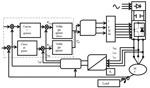
Backstepping principle of asynchronous machine is used to generate the reference current $i_{s q}^{*}$ and $i_{s d}^{*}$, representing the virtual command. And in order to ensure machine stability the control law is then adapted $V_{s d}^{*}$ and $V_{s q}^{*}$ and Figure 1 represents it.
Figure 1. Principle of backstepping control
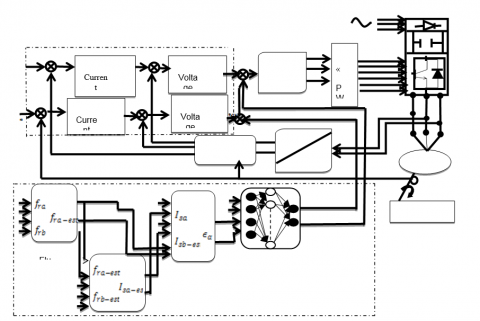
The application of neural network technique in machine control is simple and allowed the resolution of several problems related to controlling these systems. In this work with fault tolerant control, it is easy to use this technique, where the extended Kalman filter in our proposed method of FTC (FTC-EKF) is replaced by controller based on neural networks (FTC-ANN) as is illustrated in Figure 2.
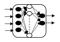
The proposed neural network is a multilayer network (4-4-2) with the architecture illustrated in Figure 3. Each neuron is connected to all neurons of the next layer by connections whose weights are randomly chosen real numbers. We notice that Wxy is the weight of the connection between neurons x and y. The following steps are necessary to obtain this ANN:
Figure 2. Principle of fault-tolerant control based on a neural network
Figure 3. Internal structure of a controller based on neural network
4.1 Artificial neural network topology
As shown in Figure 3, the proposed artificial network consists of four layers, namely: the input layer consists of four neurons, whose function is to transmit the input values that correspond to the input variables to the next layer called hidden layer. The hidden layer is characterized by four neurons. The output layer is composed of two neurons.
4.2. ANN learning stage
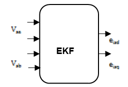
The second stage in designing the ANN is the learning process which requires a data base defining the ANN input-output mapping. This data base is mostly given under matrix form as to clarify the inputs and the desired outputs according to the Kalman filter, see Figure 4.
Figure 4. Extended Kalman filter of the proposed FTC
Despite the robustness of the Backstepping control with respect to the Cr load torque and parametric variations, she is exhausted in front of the effect of some defects. Uad is the term that must be added to the nominal control which makes up for the effect of faults on the system, it is from the outputs of the system to be ordered that this term is generated.
$U={{U}_{nom}}+{{U}_{ad}}$ (36)
$U=\left[\begin{array}{l}U_{\text {dnom }} \\ U_{\text {qnom }}\end{array}\right]+\left[\begin{array}{l}U_{\text {dad}} \\ U_{\text {qad}}\end{array}\right]$ (37)
With the expression retained from the nominal control:
$\left\{ \begin{align} & {{U}_{dnom}}=\delta {{L}_{s}}\left( {{K}_{4}}\left( {{i}_{sdref}}-{{i}_{sd}} \right)+{{i}_{sdref}}-{{F}_{d}} \right) \\ & {{U}_{qnom}}=\delta {{L}_{s}}\left( {{K}_{3}}\left( {{i}_{sqref}}-{{i}_{sq}} \right)+{{i}_{sdref}}-{{F}_{q}} \right) \\\end{align} \right.$ (38)
We can then estimate the flux:
$\left\{ \begin{align} & {{\phi }_{raest}}=\frac{1}{M}({{L}_{e}}{{\phi }_{ra}}-S{{L}_{r}}{{L}_{s}}){{I}_{as}} \\ & {{\phi }_{rbest}}=\frac{1}{M}({{L}_{e}}{{\phi }_{rb}}-S{{L}_{r}}{{L}_{s}}){{I}_{bs}} \\ \end{align} \right.$ (39)
So the calculation of the estimated currents $I_{\text {asest}}, I_{\text {bsest}}$ can get out by:
$\left\{ \begin{align} & {{I}_{asest}}=\int{{{I}_{asest}}}\left( -{{R}_{r}}{{M}^{2}}+L_{r}^{2}R{}_{s} \right)+{{\phi }_{raest}}M{{R}_{r}}/\left( S{{L}_{s}}L_{r}^{2} \right)+\frac{{{w}_{r}}M{{\phi }_{rbest}}}{S{{L}_{s}}{{L}_{r}}}+{{v}_{sa}}\frac{1}{S{{L}_{s}}} \\ & {{I}_{bsest}}=\int{{{I}_{bsest}}}\left( -{{R}_{r}}{{M}^{2}}+L_{r}^{2}R{}_{s} \right)+{{\phi }_{rbest}}M{{R}_{r}}/\left( S{{L}_{s}}L_{r}^{2} \right)-\frac{{{w}_{r}}M{{\phi }_{raest}}}{S{{L}_{s}}{{L}_{r}}}+{{v}_{sb}}\frac{1}{S{{L}_{s}}} \\ \end{align} \right.$ (40)
So the residual current error:
${{I}_{add}}=\frac{{{K}_{j}}M{{L}_{r}}}{j{{K}_{i}}}\int{\frac{-\gamma }{S{{L}_{s}}}}\left( \left[ \left( {{I}_{as}}-{{I}_{asest}} \right){{I}_{asest}} \right]+\left[ \left( {{I}_{as}}-{{I}_{asest}} \right){{I}_{asest}} \right] \right)$ (41)
So, we can deduce the constant parameters expressions as follows:
$\left\{ \begin{align} & {{\varepsilon }_{\alpha }}=\int{\alpha \left[ \left( \left( {{I}_{ds}}-{{I}_{dsest}} \right){{I}_{dsest}} \right)+\left( \left( {{I}_{qs}}-{{I}_{qsest}} \right){{I}_{qsest}} \right) \right]} \\ & {{\varepsilon }_{\beta }}=\int{\frac{\beta }{{{L}_{r}}}\left[ \left( \left( {{I}_{ds}}-{{I}_{dsest}} \right)\left( {{\phi }_{drest}}-{{I}_{dsest}} \right) \right)M+\left( \left( {{I}_{qs}}-{{I}_{qsest}} \right)\left( {{\phi }_{qrest}}-{{I}_{qsest}} \right) \right)M \right]} \\ \end{align} \right.$ (42)
The Kalman gain is given by:
$\begin{aligned} K(k+1)=& P(k+1 / k) H^{t}(k+1)[H(k\\ &+1) P(k+1 / k) H^{t}(k+1) \\ &+R(k+1)]^{(-1)} \end{aligned}$ (43)
where:
$H[K+1]=\frac{\partial h[x(t), t]}{\partial x}=\left[\begin{array}{lllll}1 & 0 & 0 & 0 & 0 \\ 0 & 1 & 0 & 0 & 0\end{array}\right]$ (44)
The updated covariance is given by:
$P(k+1 / k+1)=[1-K(K+1) H(K+1)] P(k+1 / k)$ (45)
The extended Kalman filter correction equation is described by:
$\begin{aligned} \hat{x}(k+1 / k+1) &=\hat{x}(K+1 / K) \\ &+K(K+1)\{Z(K+1)\\ &-H[\hat{x}(K+1 / K())[]]\{\}\} \end{aligned}$ (46)
4.3 ANN validation
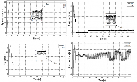
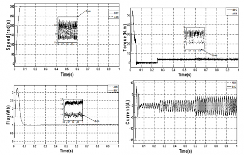
In contrast to the method used in Matlab which consists to use the learning data base for training and the remaining for the validation test. The results given by the trained network and the motor behavior are depicted in Figure 5 and 6. The test result shows the behavior of the Backstepping control structure (BSC) applied to the induction machine compared to a fault tolerant control with Kalman filter (FTC-EKF) and with neural network (FTC-ANN).
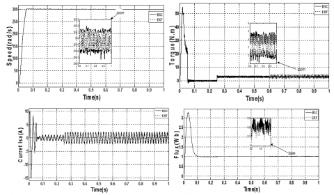
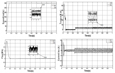
To compare the effectiveness and robustness between the proposed fault tolerant control with EKF and with ANN and the backstepping control, short circuit fault and inverter fault (cut of an arm) are introduced on both control structure (backstepping and FTC). The reference speed is fixed to 300rd/s. The MAS is started in balanced operation, we apply a load torque (3.5 N.m) at t=0.25 sec followed by defects (short circuit between turns, inverter fault) at t = 0.6 sec.
(a) Fault tolerant control based on EKF
(b) Fault tolerant control based on ANN
Figure 5. Fault tolerant control for short circuit between coils
(a) fault tolerant control based on EKF
(b) fault tolerant control based on ANN.
Figure 6. Fault tolerant control for Inverter fault (cut of an arm)
In order to show the FTC structure behavior based on ANN (FTC-ANN) for induction machine with backstepping control the system performance in steady state and transient are represented whose operation is normal then followed by a fault at t = 0.6 s. The speed responses are represented and followes its references values with a faster response with no ripple for normal operation in any case we create the default at t = 0.6 s, and during operation the MAS performance is illustrated. The machine is trained at 300 rad/s before and after the occurrence of defects and with a constant load torque of 3.5 Nm using backstepping and FTC control methods. We can notice that the implemented ANN has generated the right additive term according to the Kalman filter in the backstepping control applied to the induction motor. It is easy to filter or reduce these harmonics during the motor operating. With the backstepping control we can observe a positive ripple of the flux but with tolerant control the amplitude of ripples is acceptable for both methods (FTC-EKF) and (FTC-ANN). The main objective of a fault tolerant system is to recover dysfunctional performance close to that which it has under normal operating conditions. The fault tolerant control is used to provide a solution to the frequent problems and to reduce the costs of their treatments. The problem that arises is how to ensure a minimum level of drive system performance that is malfunctioning for example a partial or complete defect of current sensors, short circuit etc. So, we can conclude as a result that the backstepping control and FTC with Kalman filter (FTC-EKF) can give satisfactory robustness; on the other hand the tolerant control with the proposed method (FTC-ANN) can give improvement for the electromagnetic torque ripples and even for the positive ripples of the speed and flux.
5.1 Comparative study between conventional and proposed methods
Table1 summarize the main improvements of the proposed FTC-ANN compared to FTC-EKF. Figures 5 and 6 shows a comparison between the BSC conventional and proposed methods. It can be seen clearly that the ripples in torque with FTC-ANN are less than 1.87 N.m (for the short circuit fault), 2.21 N.m (for the inverter fault) and with FTC-EKF are about 2.12 N.m (for the short circuit fault), 2.65 N.m (for the inverter fault) at the same operating conditions, this can justify that the ripples are reduced to about 35% under the proposed technique. In addition, it can be seen that the magnitude of the rotor flux and speed
for FTC-FKF which has a large value of ripple, while the magnitude of the rotor flux and speed for FTC-ANN which has a minimum value of ripple.
Table 1. Comparative study between FTC-EKF and FTC-ANN
|
Fault type |
Short circuit (figure 5) |
Cut of an inverter arm (figure 6) |
|||||
|
Performance |
BSC |
EKF |
ANN |
BSC |
EKF |
ANN |
|
|
Speed |
Ripple (rad/s) |
0.43 |
0.32 |
0.22 |
0.49 |
0.3 |
0.19 |
|
Torque |
Ripple (N.m) |
3.44 |
2.12 |
1.87 |
4.02 |
2.65 |
2.21 |
|
Flux |
Ripple (Wb) |
0.0091 |
0.007 |
0.006 |
0.025 |
0.02 |
0.011 |
Neural networks (ANN) can be used to fault tolerant control of induction machine. The effectiveness of these architectures has been demonstrated by examples of simulation and satisfactory results were obtained. For the implementation of the neural network, several parametric studies were performed (choice of network type, choice of inputs, outputs choice ...). Fault-Tolerant Control is one of the most interesting industrial researches, to provide tolerance to defaults, and even to reduce defects treatment cost, thus to maintain the operation despite the appearance of defects. This paper presents a new fault-tolerant control method based on neural network that has been studied and applied to the asynchronous machine. The efficiency of the FTC control is attested and represented by the results obtained which show a marked improvement in the MAS performance even in presence of stator defects, more precisely for the reduction of fluctuations in the stator currents and the ripples of torque.
APPENDIX A
|
$z=M_{s r}-\frac{3 M_{s r}^{2}(A-B)}{2 C}$ |
|
$\lambda=z+l_{r f}$ |
|
$H=\lambda^{2}-\frac{\mathrm{z} \lambda}{2}-\frac{z^{2}}{4}$ |
|
$|\Gamma|=f_{s a}^{2} f_{s b}^{2} f_{s c}^{2}\left(\lambda^{3}-\frac{3 z^{2} \lambda}{4}-\frac{z^{3}}{4}\right)$ |
|
$d_{1}=\left(z+l_{s f}\right)^{2}-\frac{z^{2}}{4}$ |
|
$d_{2}=\frac{z\left(z+l_{s f}\right)}{2}+\frac{z^{2}}{4}$ |
|
$A=\left(l_{r f}+M_{r}\right)^{2}-\frac{M_{r}^{2}}{4}$ |
|
$B=\left(M_{r} \mathrm{L}_{r f} / 2\right)+3 M_{r}^{2} / 4$ |
|
$C=l_{r f}^{3}+3 L_{r f}^{2} M_{r}+\left(\frac{9}{4}\right) M_{r}^{2} l_{r f}$ |
|
$G=\frac{R_{r}(A-B)}{C}$ |
|
$K=\frac{M_{s r} H(A-B)}{C|\Gamma|}$ |
|
$\delta=\frac{M_{s r} R_{r}(A-B)}{C}$ |
|
$T=\frac{M_{s r}^{2} R_{r}(A-B)^{2}}{C^{2}}$ |
APPENDIX B
Table 2. Machine Parameters
|
Parameters |
Identifiers &Values |
|
Pairs poles number |
P=1 |
|
Stator frequency |
f=50Hz |
|
Stator phase resistance |
Rs=1.633Ω |
|
Rotor cage resistance |
Rr=0.93Ω |
|
Rotor inductance |
Lr=0.142H |
|
Stator cyclic inductance |
Ls=0.076H |
|
Moment of inertia |
J=0.0111Nms2 |
Acronyms
|
MAS |
: Asynchronous machine. |
|
BS |
: Backstepping. |
|
BSC |
: Backstepping control. |
|
FTC |
: Fault tolerant control. |
|
ANN |
: Artificial neural network. |
|
EKF |
: Extended kalman filter. |
SYMBOLS
|
Cr |
: Resistant torque. |
lsf |
: Stator leakage inductance. |
|
fr |
: Coefficient of friction. |
ls |
: Own inductance of a stator phase. |
|
j |
: Moment of inertia. |
lr |
: Own inductance of a rotor phase. |
|
p |
: Number of pole peers. |
Msr |
: Mutual inductance between a stator phase and a rotor phase. |
|
wr |
: Rotational speed of rotor versus stator. |
Ms |
: Mutual inductance between two stator phases. |
|
$\theta$ |
: Electric angle. |
$i_{s d}^{*}$ |
: The reference stator current on the axis d. |
|
isa,b,c |
: Stator currents. |
ew |
: Error between actual electric speed and reference speed. |
|
$\phi_{{ra.b.c}}$ |
: Rotor flux. |
$e_{\phi_{r}}$ |
: Error between rotor and reference flux module. |
|
Mr |
: Mutual inductance between two rotor phases. |
$e_{i_{s q}}$ |
: Error between the stator current on the q axis and its reference. |
|
Rs |
: Resistance of a stator phase. |
$e_{i_{s d}}$ |
: Error between the stator current on the axis d and its reference. |
|
Rr |
: Resistance of a rotor phase. |
${i_{s q}}$ |
: The stator current on the axis q. |
|
Tr |
: Rotor time constant. |
${i_{s d}}$ |
: The stator current on the axis d. |
|
$\sigma$ |
: Coefficient of dispersion of blondel. |
w* |
: Reference electric speed. |
|
$\omega$ |
: Electric speed. |
$\phi_{r}^{*}$ |
: Reference rotor flux. |
|
$\phi_{r}$ |
: Rotor flux. |
$i_{s q}^{*}$ |
: The reference stator current on the axis q. |
[1] Lall, K.P., Sabah, Baby, V.S., Chitra, T.C. (2014). A Comparative analysis of VSI & 7 level MLI fed induction motor drive with IFOC scheme and pump load. Journal of Engineering Research and Applications, 4(7): 100-107.
[2] Khadar, S., Kouzou, A., Hfaifa, A., et al. (2019). Investigation on SVM-Backsteppingsensorless control of five-phase open-end winding induction motor based on model reference adaptive system and parameter estimation. Engineering Science and Technology, an International Journal. https://doi.org/10.1016/j.jestch
[3] Layadi, N., Zeghlache, S., Djerioui, A., Mekki, H., Houari, A., Benkhoris, M.F., Berrabah, F. (2018). Interval type-2 fuzzy adaptive strategy for faulttolerant control based on new faulty model design: Application to DSIM underbroken rotor bars fault. AMSE Journals, Modelling, Measurement and Control A, 91(4): 212-221.
[4] Niemann, H., Stoustrup, J. (2004). Passive fault tolerant control of a double inverted pendulum - a case study. Control Engineering Practice, 13: 1047-1059. https://doi.org/10.1016/j.conengprac.2004.11.002
[5] He, J.J., Qi, R.Y., Jiang, B., Qian, J.S. (2015). Adaptive output feedback fault-tolerant control design for hypersonic flight vehicles. Journal of the Franklin Institute, 352: 111-1835. https://doi.org/10.1016/j.jfranklin.2015.01.016
[6] Morse, W.D., Ossman, K.A. (1990). Model following reconfigurable flight control system for the AFTI/F-16. Journal of Guidance, Control, and Dynamics, 13(6), 969-976. https://doi.org/10.2514/3.20568
[7] Qin, W., Kumar, R., Huang, J., Liu, H. (2008). A Framework for Fault-Tolerant Control of Discrete Event Systems. IEEE Transactions on Automatic Control, 53(8): 1839-1849. https://doi.org/10.1109/TAC.2008.929388
[8] Kowalski, C.T., Orlowska-Kowalska, T. (2003). Application of Neural Networks for the Induction Motor Faults Detection. Tran of IMACS Mathematics and Computers in Simulation, 63(3-5): 435-448.
[9] Mohanapriya, P., Umadevi, K. (2018). Direct Torque Control of Three Phase Induction Motor Using Neural Network-Fuzzy Logic Techniques. International Journal of Development Research, 8(1): 18233-18239.
[10] Benbouhenni, H. (2018). Improved Switching Selection for Dtc Of Induction Motor Drive Using Artificial Neural Networks. ActaElectrotechnica et Informatica, 18(1): 26-34. https://doi.org/10.15546/aeei-2018-0004
[11] Jia, C.X., Qiu W.N., Pu, X.Z. (2016). New Residual Current Compensation Method for Single-Phase Grounding Fault in Power Network Based on Capacitive Current Detection and Analysis. AMSE Journals, Modelling A, 89(1): 205-223.
[12] Fan, S., Zou, J. (2012). Sensor fault detection and fault tolerant control of induction motor drivers for electric vehicles. IEEE 7th International Power Electronics and Motion Control Conference - ECCE Asia, Harbin, China, 1306-1309. https://doi.org/10.1109/IPEMC.2012.6259046
[13] Mini, V.P., Ushakumari, S. (2014). Rotor fault detection and diagnosis of induction motor using fuzzy logic. AMSE JOURNALS 2014-Series: Modelling A, 87(2), 19-40.
[14] Jiang, J., Xiang, Y. (2012). Fault-tolerant control systems: A comparative study between active and passive approaches. Annual Reviews in Control, 36: 60-72. https://doi.org/10.1016/j.arcontrol.2012.03.005