Antonio Kido Cruz![]() | Teresa Kido Cruz
| Teresa Kido Cruz![]() | Felipe Andoni Luna Campos*
| Felipe Andoni Luna Campos*![]()
OPEN ACCESS
The goal of this paper is to estimate the percentage structure of electricity generation by type of technology in Mexico for the period 1992-2016. Modern portfolio theory and the capital asset pricing model of Sharpe and Litner were used. Results show that using only portfolio theory is not possible to find non-negative percentages in all the technologies. When a risk-free asset is included, there is a region where all technologies have a positive participation in electricity generation. The efficient frontier is found at 20% for wind technology share and for the rest of technologies, shares are almost equally – distributed among them.
electricity generation, optimal theory, efficient frontier
One of the programs for electricity generation forecast by the Centro Nacional de Energía (CENACE-National Center for Energy Control) based on cost structure by technology type and existing capacity is constituted by the optimization model based on the branch and bound algorithm (Branch and Bound). The PLEXOS option of this algorithm is solved by linear programming (LP), that is to say, without the existence of integrity conditions over the variables [1].
Taking into account installed capacity, in 2017 structure according to electricity generation technology behaved as follows: for combined-cycle (CC) 50%; for thermoelectric power (TCC) 19.4%; for carboelectric power (CAR) 9.3%; of hydroelectric power (HIDRO) 9.7%; of nuclear generation (NUC) 3.3%; of wind power (EOLO) 3.2% and, of geothermal and biofuel technology 4.9%. For 2032, CENACE's energy mix is estimated as follows: of combined cycle 41.9%; of conventional thermoelectric power 10.1%; of carboelectric power 3.2%; of hydroelectricity 11.4%; geothermal energy 1.5%; of nuclear power 4.4%; of wind power 14.6%, and the remaining being a combination of geothermal, solar photovoltaic, biomass and efficient cogeneration.
Purpose of this work is to contrast cost structure per forecasted technology for the year 2032 using the least-cost method (currently used by CENACE) with option of mean-variance approach for Mexico. To this effect, the efficient frontier of asset portfolio will be generated according to the return-risk pair. This description is due to the approach goal which is based on obtaining the efficient technology portfolio implying to expose society to the risk minimum level necessary related to electricity generation.
At international level and especially during the last decade, it is possible to find a significant number of releases on the same topic [2-11].
Nevertheless, in Mexico, just four papers with the same subject are known. Auwerbach's work reveals that portfolio's return (the set of percentages assigned to each type of energy) for 2010 (foreseen with 2002 data) under the lower cost concept of electricity generation (commonly used by the Comisión Federal de Electricidad) which, theoretically speaking, is far from belonging to the group of efficient portfolios and a cost of 4.8 dollar cents/kWh was estimated. Optimal portfolio (based on mean-variance approach) offers a considerable improvement. Without risk of increase, this portfolio decreases to 3.6-dollar cents/kWh (1/0.28), a reduction of 25%- or 1.2-dollar cents/kWh [12].
Beltran [13] reports that, in a forecast (carried out in 2008) of a portfolio by technology type of electricity levelized cost (for the year 2017) of Mexican authorities on these issues, based on the lower cost method, electricity generation system will depend 60% on natural gas-fueled combined cycle power plants to satisfy electricity demand in the country. Instinctively, it points out that this percentage represents a remarkably high reliance on fossil fuels source and, therefore, a high level of accompanying risk is implied. On the other hand, general expected return has a generation cost of 76.66 $/MWh and a portfolio risk of 0.22. The optimal portfolio with a cost level equal to that of the objective shows a possibility of having the same cost profile as the portfolio objective, but they achieve a lower level of risk exposure. In this case the risk factor is reduced from 0.22 to 0.124.
Gómez-Ríos [14] shows that geothermal and hydroelectric plants are key technologies to reduce risk due to fuel price volatility. Wind energy is risky in terms of completed capacity. Nuclear and coal plants are stable concerning capacity and operating costs. Thermal and gas technologies are the most vulnerable to variability in fuel prices.
Gómez-Ríos and Juárez-Luna [15] estimate total levelized cost of generation with Externalities (CTNGE from Spanish acronym of Costo Total Nivelado de Generación con Externalidades - Total Levelized Cost of Generation with Externalities) of three base-load technologies: coal thermoelectric, combined cycle and nuclear power plant. Monte Carlo simulation is used to forecast probability densities of the CTNGE.
Portfolio theory is used to find technologies mix providing the least risky CTNGE and with the least average. Nuclear plant is found to have the lowest CTNGE. Being the coal-fired thermoelectric the technology with the extensive and riskiest CTNGE. In electricity generation, analysis suggests that it would be most desirable to leave out coal-fired thermoelectric plant and focus on two technologies: combined cycle and nuclear power plant, assigning a higher participation to the latter. One of this work limitations is that CTNGE's probability densities estimated through Monte Carlo simulation depend on used data. Echeverría et al. [16] also point out it would be more convenient to choose nuclear technology for electricity generation based on actual options methodological criteria.
In finance, investors use portfolio theory to minimize the risk and maximize the return of their portfolio by diversification. Some theories can be used in electricity generation planning to evaluate the addition of each new alternative on the basis of its contribution to the overall risk and cost of the generation mix and not on its stand – alone cost [5].
There are electricity generation technologies showing high correlations, according to their fuel and/or operation and maintenance costs among them (more substitutes) such as CC gas plants as well as those of fossil fuel and coal; likewise, other technologies with almost nil correlations (more complementary) can be identified, such as those using fossil fuels with those operating based on nuclear energy or with solar and wind technologies. Besides, there is also a possibility of technologies with a negative correlation, such as it is the case between Biomass and fuel derivatives [12].
These considerations are the basis for implementing optimization processes through theories involving mean-variance use. Having this information, one of the most interesting questions in the electricity sector area is the following: what changes may be feasible in the energy mix of a country or region allowing to win in one of both dimensions (risk-return) of optimal portfolio without harming the other? Of course, among all efficient portfolios, the optimal choice depends on preferences of the energy policy consultant [17].
3.1 Set of efficient portfolios when all values are at risk
On the Markowitz's portfolios optimization theory formalism, the main elements are a set of m assets. From each one of them arises a series in time of T data (measured in investment units); in the case of investment portfolios, they correspond to assets' closing prices. Thus, from which we obtain returns T-1, following Eq. (1):
$r_t=\left(P_t-P_{t-1}\right) / P_{t-1}($ dimensionless $)$ (1)
These returns T-1 form a series in time having those same elements number.
3.2 Portfolios optimization problem
Markowitz's attainment was to relate standard deviation with the risk, giving to the latter the task of assigning a quantitative measure. The problem of reducing the risk of a portfolio, given an expected return value, can be mathematically written as an optimization problem with m-dimensional constraints that is given by:
$\min _{\underline{x}_p} F\left(\underline{x}_p\right)$ (2)
s.t. $E\left(\underline{x}_p\right)=E_p$ (3)
$\sum_{i=1}^m x_i=1$ (4)
Solution to this problem is $\underline{x}_p^*$, in such a way that it complies with being the minimum of all values of objective function F and additionally with the constraints that $E\left(\underline{x}_p^*\right)=E_p$ and $\sum_{i=1}^m x_i^*=1$.
We can change the optimization problem with m - dimensional constraints to a problem with no constraints m + 2 - dimensional, using the Lagrange multipliers:
$\min _{\left(\underline{x}_p, \lambda_1, \lambda_2\right)} L:=F\left(\underline{x}_p\right)-\gamma_1 g_1\left(\underline{x}_p\right)-\gamma_2 g_2\left(\underline{x}_p\right)$ (5)
where, g1 and g2 are defined using problem constrains:
$g_1\left(\underline{x}_p\right):=E\left(\underline{x}_p\right)-E_p$ (6)
$g_2\left(\underline{x}_p\right):=\sum_{i=1}^m\left(\underline{x}_p\right)_i-1$ (7)
3.3 Solving the problem with no constrains
Conditions necessary to find a stationary point for the problem with no constrains are given by:
$\nabla_{\left(x, \lambda_1, \lambda_2\right)} L=0$ (8)
The $\nabla_{\left(\underline{x}, \lambda_1, \lambda_2\right)}$ operator means that we will perform m+2 partial derivatives of L, we will accommodate them as components of a column vector and we equalize them to a column vector with zeros as components:
$\frac{\partial}{\partial x_1} L=0 \cdots \frac{\partial}{\partial x_m} L=0 \cdot \frac{\partial}{\partial \lambda_1} L=0, \frac{\partial}{\partial \lambda_2} L=0$ (9)
To find the stationary point $\left(\underline{x}_p^*, \lambda_1^*, \lambda_2^*\right)$ is necessary to solve the algebraic equations system resulting from the solution of previous partial derivatives, which can be explicitly written as follows:
$0=\sum_{i=1}^m x_j \sigma_{i j}-\gamma_1 E_i-\gamma_2 \cdot 1, i=1, \ldots m$ (10)
$0=E-\sum_{i=1}^m x_i E_i$ (11)
$0=1-\sum_{i=1}^m x_i$ (12)
Please note that we have omitted bars and asterisks from our previous notation so that $\left(\underline{x}_p^*\right)_j=x_j, \gamma_1^*=\gamma_1 y \gamma_2^*=\gamma_2$.
Here we can see that there are m+2 equations with m+2 unknowns instead of a system of partial differential equations. For convenience we will go to the matrix form of the problem:
$\left(\sigma \underline{x}^T\right)_i-\left(\gamma_1 \underline{E}\right)_i-\left(\gamma_2 \underline{1}\right)_i=0, i=1, \ldots, m$ (13)
$0=E-\underline{x}^T \underline{E}$ (14)
$0=1-\underline{1}^T \underline{x}$ (15)
The weights vector (column) $\underline{x}=\left(x_1, x_2, \ldots, x_m\right)^T$ is the vector that contains the percentages (which will be a main part of the optimization problem together with the Lagrange multipliers $\lambda_1$ and $\lambda_2$. We also specify that $\underline{x}^T=\left(x_1, x_2, \ldots, x_m\right)$ is a row or line vector of m inputs with the same components as $\underline{x}$. Here $\underline{E}=\left(\mu_1, \ldots, \mu_m\right)^T$ is the column vector containing the averages or means of historical data. On the other hand, $\underline{1}=(1, \ldots, 1)^T$ is the column vector of m components that only has entries with value 1.
Making use of matrix notation to find the solution to the equations system:
$\sigma \underline{x}-\gamma_1 E-\gamma_2 \underline{1}=\underline{0}$ (16)
where, $\underline{0}^T=(0, \ldots, 0)^T$ is a column vector with zeros in all its inputs (components). We define the inverse matrix of $\sigma$ as the one having the vij components:
$\left[\sigma^{-1}\right]_{i j}=v_{i j}$ (17)
Analytically speaking (meaning, beyond computers field) for the inverse matrix of σ, to exist, sufficient condition that must be met is that determinant must be different to zero.
Therefore, by multiplying Eq. (16) by the inverse matrix we have:
$\sigma^{-1} \sigma \underline{x}-\gamma_1 \sigma^{-1} \underline{E}-\gamma_2 \sigma^{-1} \underline{1}=\sigma^{-1} \underline{0}$ (18)
note that $\sigma^{-1} \sigma=1_{m \times m}$, where $1_{m \times m}$ is the identity matrix that has ones on the diagonal and zeros in all the remaining entries. By multiplying inverse matrix by a vector, we obtain another same dimension vector as the initial one. And finally, we observe the simple multiplication $\sigma^{-1} \underline{0}=\underline{0}$ on the equation's right side.
Finally, the result of the above equation is:
$\underline{x}-\gamma_1 \sigma^{-1} \underline{E}-\gamma_2 \sigma^{-1} \underline{1}=\underline{0}$ (19)
note that if $\gamma_1$ and $\gamma_2$ were known, then we would immediately have the solution values since vector $\underline{E}$ and matrix $\sigma^{-1}$ are known or calculable from the problem data. Therefore, our task from now on is to find $\gamma_1$ and $\gamma_2$.
We can write for the k-th component of Eq. (19) as:
$x_k=\gamma_1 \sum_{j=1}^m v_{k j} E_j+\gamma_2 \sum_{j=1}^m v_{k j}, k=1, \ldots m$ (20)
Multiplying the previous equation by Ek and adding on k we have:
$\sum_1^m x_k E_k=\gamma_1 \sum_1^m \sum_1^m v_{k j} E_j E_k+\gamma_2 \sum_1^m \sum_1^m v_{k j} E_k$ (21)
which in matrix notation is:
$\underline{x}^T \underline{E}=\gamma_1 \underline{E}^T \sigma^{-1} \underline{E}+\gamma_2 \underline{1}^T \sigma^{-1} \underline{E}$ (22)
on this equation's right side we will use the definition of the return expected value of a portfolio in its matrix form, $\underline{x}^T \underline{E}=E_p$, where Ep is a problem's data, thus:
$E_p=\gamma_1 A+\gamma_2 B$ (23)
where two of the three Merton scalars have been defined:
$A=\underline{E}^T \sigma^{-1} \underline{E}, B=\underline{1}^T \sigma^{-1} \underline{E}$ (24)
which can be calculated from the variance-covariance inverse matrix and from the means vector; therefore, they are values that can be considered problem's data. On the other hand, if we carry out the contraction operation, that is the sum of all the vector components xk, we obtain:
$\sum_1^m x_k=\gamma_1 \sum_1^m \sum_1^m v_{k j} E_j+\gamma_2 \sum_1^m \sum_1^m v_{k j} E_k$ (25)
This also has its matrix form, represented by:
$\underline{1}^T \underline{x}=\gamma_1 B+\gamma_2 C$ (26)
where we can see that the third scalar, obtained from Merton is:
$C \equiv \sum_1^m \sum_1^m v_{k j}$ (27)
Left side of this Eq. (26) equals 1 as it is the budget constraint to which the problem is subject, and therefore:
$1=\gamma_1 B+\gamma_2 C$ (28)
Thus, a system of two equations with two unknowns is formed $\left(\gamma_1, \gamma_2\right)$ whose solution is:
$\gamma_1=\frac{(E C-B)}{D}, \gamma_2=\frac{(A-E B)}{D}$ (29)
This solution can be seen immediately if we use Cramer's formula and if, besides, for this solution to exist, we ask that the discriminant $B C-A^2=D \neq 0$.
Once obtained $\left(\gamma_1, \gamma_2\right)$ we substitute in 1 system to obtain the solution:
$\begin{aligned} & x_k=\frac{E \sum_1^m v_{k j}\left(C E_j-A\right)+\sum_1^m v_{k j}\left(B-A E_j\right)}{D} \\ & k=1, \ldots, m \\ & \end{aligned}$ (30)
3.4 Efficient frontier
Graphically, the efficient frontier is described by all those points on plane $\sigma-E$ where for a certain given value of Ep we find minimum $\sigma_p$ that a linear combination with weights $\underline{x}_p$ can give.
To obtain the geometric place in R2 with axis of the abscissae equal to the risk $\sigma$ and the ordinates axis equal to portfolio return Ep, we construct an expression that relates these two quantities multiplying (10) by xi and adding of $i=1, \ldots, m$:
$\sum_{i=1}^m \sum_{j=1}^m x_i x_j \sigma_{i j}=\gamma_1 \sum_{\substack{1 \\ i=1,...m}}^m x_i E_i+\gamma_2 \sum_1^m x_i$ (31)
Left side of this expression is the portfolio variance definition, that is to say, $\sigma^2\left(x_p\right)$, while on the right side we obtain $\gamma_1$ multiplying by Ep which is the expected value of the portfolio return and $\gamma_2$, the budgets’ equation which is 1. From which we obtain:
$\sigma^2\left(x_p\right)-\frac{1}{C}=\frac{C}{D}\left(E_p-\frac{A}{C}\right)^2$ (32)
If C and D are greater than zero, then the right side of Eq. (32) will always be positive since it is written in terms of $\left(E_p-\frac{A}{C}\right)^2 \geq 0$. When $E_p=\frac{A}{C}$ this term will be zero and therefore $\sigma^2\left(x_p\right)=\frac{1}{C}$.
We define $\underline{E} \equiv \frac{A}{C}$ as the minimum expected value of a portfolio that has the minimum variance $\underline{\sigma}^2 \equiv \frac{1}{C}$.
Defining $\underline{x}_k$ so that it is the proportion of the minimum variance portfolio invested in the asset $k^{t h}$, then it is necessary to redefine:
$\underline{x}_k=\frac{\sum_1^m v_{k j}}{C}, k=1, \ldots, m$ (33)
However, it is usual to present the frontier in the standard deviation plane of the mean instead of the mean-variance plane, so its geometric representation is represented will remain as:
$\frac{\sigma^2}{\frac{1}{C}}-\frac{\left(E-\frac{A}{C}\right)^2}{\frac{D}{C}}=1$ (34)
According to analytical geometry, this equation represents a hyperbola that meets and confirms conditions of an efficient portfolio with minimum variance in $E \equiv \frac{A}{C}$ and a minimum variance of $\underline{\sigma}^2 \equiv \frac{1}{C}$.
3.5 Non-negative weights
According to literature [18], both the optimal theory model and the capital assets pricing model [19] indicate that portfolios generated with positive investment percentages will have a characteristic of being efficient within the mean-variance relationship.
However, these types of portfolios (all the positive weights) are not so common to obtain, especially if data from assets' historical series are used. In the best-case scenario, their results indicate that, only it is possible to identify a single segment of the efficient frontier where all are no-negative weights.
Written parametrically, Markowitz can be transcribed as follows:
$\max \left\{t E^{\prime} x-\frac{1}{2} x^{\prime} \sigma x \mid 1^{\prime} x=1\right\}$ (35)
where, t is a scalar parameter, x is the portfolio's n-vector of weights, and $1^{\prime} x=1$ is the budget constraint. Solution to this problem in terms of parameter t for x and t is:
$x(t)=\frac{\sigma^{-1} 1}{C}+t\left[\sigma^{-1}\left(E_p-\frac{1 A}{C}\right)\right]$ (36)
$\lambda(t)=-\frac{1}{C}+\frac{t A}{C}$ (37)
where, A, B and C are the Merton scalars from the previous section. Now let us define:
$h_0=\frac{\sigma^{-1} 1}{C}$ (38)
$h_1=\sigma^{-1}\left(E_p-\frac{1 A}{C}\right)$ (39)
So, portfolio weights can be expressed as:
$x(t)=h_0+t h_1$ (40)
It is clearly seen from this equation if we observe each component separately, then:
$x_i(t)=\left(h_0\right)_i+t\left(h_1\right)_i, i=1, \ldots, m$ (41)
that if $h 1_i>0$, then $x_i(t)$ increases as t raises and it will be positive since $t \geq\left(h_0\right)_i /\left(h_1\right)_i$.
It is possible to determine a maximum dimension and a minimum dimension for t's values in such a way that we can guarantee existence of positive weights:
$t_l=\max \left\{-\left(h_0\right)_i /\left(h_1\right)_i \mid\right.$ for all $i$ with $\left.\left(h_1\right)_i>0\right\}$ (42)
$t_u=\min \left\{-\left(h_0\right)_i /\left(h_1\right)_i \mid\right.$ for all $i$ with $\left.\left(h_1\right)_i<0\right\}$ (43)
From where it is not difficult to conclude that:
$x_i(t) \geq 0$ for all $i$ with $\left(h_1\right)_i>0$ and for all $t \geq t_l$ (44)
$x_i(t) \geq 0$ for all $i$ with $\left(h_1\right)_i<0$ and for all $t<t_\mu$ (45)
note that for $x(t)$ to be positive in all its components for some t it is necessary that:
$\left(h_0\right)_i \geq 0$ for all $i$ so that $\left(h_1\right)_i=0$ (46)
This implies that $x(t)>0$ alone and if $t_l \leq t \leq t_u$ and the above constraint is complied with literature [18]. From here it is easy to obtain a strong conclusion that if $t_l>t_u$ there are no positive components of $x(t)$.
3.6 Used information
Total levelized annual cost includes three areas: a) cost per investment; b) cost per fuel and c) cost per operation and maintenance (includes cost for water consumption). From 1992 to 2011, information was provided by Taboada González et al. [20]. This information is in Mexican pesos and it was developed with information from COPAR (Spanish acronym of Costs and Reference Parameters for Investment Project Formulation in the Electrical Sector). From 2012 to 2016, the same Taboada procedure was followed except that information was stated in dollars, so the peso-dollar exchange rate was applied to convert to pesos the annual averages obtained from each generation technology. The calculation is based on the COPAR's 2012 and 2015 documents.
4.1 Results using levelized the cost inverse and optimal portfolio theory with annual information from 1992 to 2011
It is important to remember that criterion for finding all positive weights is met when $t_l>t_u$. in the case of the range of the analyzed sample, the result was that $t_l<t_u$ (0.35 is not lower than 0.11) so it is not possible to find an efficient portfolio having only non-negative values (Refer to Appendix 1 for an extended review of the calculations to maximize and minimize the risk of the investment portfolio in electricity assets in this study). Results are shown in Table 1.
From Table 1, it can be seen that only a value of t=0.2345 has been taken for the test of formula in the third column. The first column is the h0 vector, the second column is the h1 vector, the third column is the x(t) vector evaluated at t=0.2345, fourth, fifth and sixth columns are $-\left(h_0\right)_i /\left(h_1\right)_i$; however, to solve certain problems, in excel we have redefined some cells with the NA value according to the h1 sign in the second column, to obtain the MAX (maximum) and MIN (minimum) values correctly.
Therefore, once we are convinced that by simply using Markowitz's Theory it is not possible to obtain all positive values, we proceed with calculation of the efficient frontier. Whence it follows that portfolio presents the minimum risk when E=6.8% and the risk is $\sigma$=9.2%. Likewise, we obtain that x vector has the weights for this return and risk:
$x=\left\{\begin{array}{c}-24.5 \%, 60.8 \%, 24.4 \% \\ -22.3 \%, 10.1 \%, 16.8 \%, 34.8 \%\end{array}\right\}$ (47)
Since we do not have a logical interpretation for a negative weight in this application, we must look for an option to solve this problem. Nevertheless, the same theory presents several options. One of them is to consider that one of the assets can be deemed as a risk-free asset.
4.2 Results using wind technology as a risk-free technology
Assuming that wind technology can be modeled as a risk-free technology [3, 16], which implies assuming that correlation between variations of electricity generation through clean sources related to the remaining is equal to zero, it is possible to find a range for the risk-return pair where all weights are positive, as can be seen in Table 2.
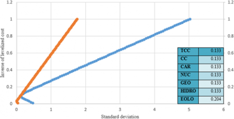
Results in Table 2 and Figure 1, indicate that there is a region where risk-free technology takes values of the expected value between 0.04 and 0.06 and the investment weights are all positive. For the remainder of the spectrum, there is at least one negative value in the series of x vector.
In the region of values all positive for x vector, we highlight when the 0.06 value is taken, in this scenario, wind technology (risk-free by assumption) finds a 0.20 value and for the remainder of technologies, the value is distributed nearly equally between them at a 0.13 value.
This would be the scenario more consistent with the Mexican reality according to installed capacity of each technology, but even so, it is quite contrasting with structure programmed by CENACE for both 2016 and its forecast for the year 2032. This relationship generates the following presentation of the efficient frontier.
Figure 1. Efficient frontier considering a risk-free asset
Table 1. Criterion to find positive weights in model with risky assets
|
$h_0$ |
$h_1$ |
$x(t)=h_0+t h_1$ |
$-\left(\boldsymbol{h}_0\right)_i /\left(\boldsymbol{h}_1\right)_i$ |
$-\left(\boldsymbol{h}_0\right)_i /\left(\boldsymbol{h}_1\right)_i$ |
$-\left(\boldsymbol{h}_0\right)_i /\left(\boldsymbol{h}_1\right)_i$ |
$-\left(\boldsymbol{h}_0\right)_i /\left(\boldsymbol{h}_1\right)_i$ |
|
-0.2 |
2.23 |
0.27 |
0.10 |
0.1 |
0.10 |
NA |
|
0.6 |
-0.68 |
0.44 |
0.88 |
NA |
0.88 |
0.88 |
|
0.2 |
-1.30 |
-0.06 |
0.18 |
NA |
0.18 |
0.18 |
|
-0.2 |
0.62 |
-0.07 |
0.35 |
0.35 |
0.35 |
NA |
|
0.1 |
-0.85 |
-0.10 |
0.11 |
NA |
0.11 |
0.11 |
|
0.1 |
1.42 |
0.50 |
-0.11 |
-0.11 |
-0.11 |
NA |
|
0.34 |
-1.43 |
0.01 |
0.24 |
NA |
0.24 |
0.24 |
|
- |
- |
- |
MAX= |
0.35 |
MIN= |
0.11 |
Source: Own elaboration based on experiment’s results
Table 2. Percentages with non-negative weights in the model that includes a risk-free technology
|
E |
Riskless S |
Risky S |
CC |
TCC |
CAR |
NUC |
HIDRO |
GEO |
EOLO |
|
0.01 |
0.036 |
0.471 |
-0.088 |
-0.088 |
-0.088 |
-0.088 |
-0.088 |
-0.088 |
1.53 |
|
0.02 |
0.018 |
0.418 |
-0.044 |
-0.044 |
-0.044 |
-0.044 |
-0.044 |
-0.044 |
1.265 |
|
0.03 |
0 |
0.365 |
0 |
0 |
0 |
0 |
0 |
0 |
1 |
|
0.04 |
0.018 |
0.314 |
0.044 |
0.044 |
0.044 |
0.044 |
0.044 |
0.044 |
0.735 |
|
0.05 |
0.036 |
0.263 |
0.088 |
0.088 |
0.088 |
0.088 |
0.088 |
0.088 |
0.47 |
|
0.06 |
0.054 |
0.215 |
0.133 |
0.133 |
0.133 |
0.133 |
0.133 |
0.133 |
0.204 |
|
0.07 |
0.072 |
0.172 |
0.177 |
0.177 |
0.177 |
0.177 |
0.177 |
0.177 |
-0.061 |
|
0.08 |
0.091 |
0.138 |
0.221 |
0.221 |
0.221 |
0.221 |
0.221 |
0.221 |
-0.326 |
|
0.09 |
0.109 |
0.12 |
0.265 |
0.265 |
0.265 |
0.265 |
0.265 |
0.265 |
-0.591 |
|
0.1 |
0.127 |
0.127 |
0.309 |
0.309 |
0.309 |
0.309 |
0.309 |
0.309 |
-0.856 |
Source: Own elaboration based on experiment’s results.
To discuss the results of the research, it will be necessary to refer to Table 3, which presents the evidence derived from the numerical experiments in three scenarios:
Scenario A: Portfolio optimization with a CAPM approach (Wind technology as the risk-free asset) using CENACE's energy mix projection for the year 2017.
Scenario B: Portfolio optimization with a CAPM approach (Wind technology as the risk-free asset) using CENACE's energy mix projection for the year 2032.
Scenario C: Portfolio optimization with a CAPM approach (Wind technology as the risk-free asset) using a self-calculated distribution of CENACE's energy mix.
Table 3. Portfolio optimization scenarios using the CAPM model
|
Scenario |
E |
σ |
CC |
TCC |
CAR |
NUC |
HIDRO |
GEO |
EOLO |
|
A |
10.8 |
12.56 |
50.20 |
19.40 |
9.30 |
3.30 |
9.70 |
4.90 |
3.20 |
|
B |
14.90 |
12.59 |
41.90 |
10.1 |
3.20 |
4.40 |
11.40 |
1.56 |
14.6 |
|
C |
6.0 |
5.4 |
13.30 |
13.30 |
13.30 |
13.30 |
13.30 |
13.30 |
20.4 |
Source: Own elaboration based on experiment’s results.
Going deeper into the proposed analysis, it can be observed that for the year 2017 and taking into account installed capacity, structure per electricity generation technology behaved as follows: 50.20% for combined-cycle (CC); 19.4% for thermoelectric power (TCC); 9.3% for carboelectric power (CAR); 9.7% of hydroelectric power (HIDRO); 3.3% of nuclear generation (NUC); 3.2% of wind power (EOLO) and; 4.9% of geothermal technology and biofuel. For this combination, return on portfolio was 10.8% with an associated risk of 12.56%.
In this same vein, for the year 2032, CENACE's energy mix is forecasted as follows: 41.9% of combined cycle; 10.1% of conventional thermoelectric power; 3.2% of carboelectric power; 11.4% of hydroelectricity; 1.56% geothermal; 4.4% nuclear; 14.6% of wind power and, the remainder, a combination of geothermal, solar photovoltaic, biomass and efficient cogeneration. With this combination, return on portfolio rises to 14.9% but with an associated risk of 12.59%. It is noted that for a same level of risk associated to the energy mix, profitability maximization (or cost decrease) is lower.
However, for scenario C, it is possible to identify that the proposed energy combination is feasible in relation to the future projections made by CENACE, the risk-return levels are acceptable, and it also weighs a 250% increase in clean energy generation compared to scenarios A and B. The aforementioned would help preserve Mexico's energy sovereignty while striving to reduce pollution levels in the environment.
In this study, historical series of electricity levelized costs were obtained for seven technologies, including investment costs, fuel costs, and operation and maintenance costs for the years from 1992 to 2016. These series were transformed into the inverse of cost to apply optimal portfolio theory and the capital asset pricing model. With the Markowitz mean-variance model, an optimal portfolio solution could not be found where values assigned to participation weighting in electricity generation were all positive; therefore, obtaining the efficient frontier lacks a significant interpretation in terms of analyzed context. When the model considering a risk-free asset is used, a region where weights are all positive is found and, consequently, it is possible to obtain the efficient frontier for the various technologies, however, this solution distributes almost in the same proportion (0.13) the weight for six of the technologies used and estimates the clean technology participation at 0.20.
It is important to emphasize that main finding of this research is the fact of having carried out the analytical development of the portfolio frontier applied to the case of real assets. However, one of the main limitations related to international literature was failure to include inequality constraints additional to those essential in Markowitz's approach. Additional constraints taking into account forecast of risk future values based on probability distributions (Montecarlo techniques) and/or GARCH* (*From English acronym of Generalized Autoregressive Condition Heteroscedastic) estimation techniques representing research future avenues.
To perform the optimization calculations from the Markowitz approach, a database is used that includes electricity levelized costs for each type of energy, as shown in Table A1.
The inverse prices are then calculated to be theoretically consistent with the optimization in the sense of Markowitz and obtain a proper interpretation of the numerical experiment results, refer to Table A2.
Table A3 displays the annual returns for each asset type, which serve as the foundation for portfolio optimization in the ongoing study.
Table A1. Time series of electricity levelized costs
|
Year |
TCC |
CC |
CAR |
NUC |
GEO |
HIDRO |
EOLO |
|
1992 |
290.64 |
137.63 |
177 |
195.81 |
175.93 |
178 |
545.69 |
|
1993 |
382.3 |
134 |
166 |
171.7 |
164 |
177 |
466.16 |
|
1994 |
413.24 |
144 |
171 |
186.06 |
164.55 |
199 |
550.31 |
|
1995 |
669.32 |
185.69 |
229.84 |
354.06 |
300.61 |
297 |
919.16 |
|
1996 |
794.23 |
218.15 |
261 |
457.73 |
396.56 |
407 |
905.28 |
|
1997 |
806.03 |
210 |
289 |
472.41 |
425.51 |
469 |
812.19 |
|
1998 |
869.83 |
235 |
329 |
444.45 |
312.39 |
541 |
841.98 |
|
1999 |
899.83 |
280 |
362 |
513.36 |
359.63 |
612 |
706.87 |
|
2000 |
989 |
305 |
396 |
536 |
367.05 |
661 |
662.61 |
|
2001 |
1078 |
330 |
430 |
559.53 |
374.47 |
709 |
595.15 |
|
2002 |
853.7 |
347.75 |
470 |
564.49 |
383.59 |
670 |
613.49 |
|
2003 |
1047 |
414 |
586 |
732.82 |
491 |
866 |
652.42 |
|
2004 |
1157.18 |
495 |
602 |
488 |
518.29 |
919 |
605.78 |
|
2005 |
1306 |
593 |
641 |
500 |
555 |
989 |
584.62 |
|
2006 |
1561 |
702 |
584 |
539.46 |
594 |
1059 |
596.63 |
|
2007 |
1621 |
722 |
688.23 |
647.41 |
642.01 |
1219 |
618.36 |
|
2008 |
1860 |
843 |
798 |
787.36 |
898 |
1304 |
805.1 |
|
2009 |
2497 |
1058.26 |
1162.81 |
1743.25 |
1186 |
1711 |
836.1 |
|
2010 |
2468 |
1098 |
1065 |
1229 |
1181.21 |
1635 |
830.03 |
|
2011 |
1827.56 |
794 |
662 |
1187.21 |
1180.8 |
1214.24 |
1032.67 |
Source: Own elaboration based on CENACE's official reports.
Table A2. Time series of inverse levelized electricity costs
|
Year |
TCC |
CC |
CAR |
NUC |
GEO |
HIDRO |
EOLO |
|
1992 |
0.0034 |
0.0073 |
0.0056 |
0.0051 |
0.0057 |
0.0056 |
0.0018 |
|
1993 |
0.0026 |
0.0075 |
0.0060 |
0.0058 |
0.0061 |
0.0056 |
0.0021 |
|
1994 |
0.0024 |
0.0069 |
0.0058 |
0.0054 |
0.0061 |
0.0050 |
0.0018 |
|
1995 |
0.0015 |
0.0054 |
0.0044 |
0.0028 |
0.0033 |
0.0034 |
0.0011 |
|
1996 |
0.0013 |
0.0046 |
0.0038 |
0.0022 |
0.0025 |
0.0025 |
0.0011 |
|
1997 |
0.0012 |
0.0048 |
0.0035 |
0.0021 |
0.0024 |
0.0021 |
0.0012 |
|
1998 |
0.0011 |
0.0043 |
0.0030 |
0.0022 |
0.0032 |
0.0018 |
0.0012 |
|
1999 |
0.0011 |
0.0036 |
0.0028 |
0.0019 |
0.0028 |
0.0016 |
0.0014 |
|
2000 |
0.0010 |
0.0033 |
0.0025 |
0.0019 |
0.0027 |
0.0015 |
0.0015 |
|
2001 |
0.0009 |
0.0030 |
0.0023 |
0.0018 |
0.0027 |
0.0014 |
0.0017 |
|
2002 |
0.0012 |
0.0029 |
0.0021 |
0.0018 |
0.0026 |
0.0015 |
0.0016 |
|
2003 |
0.0010 |
0.0024 |
0.0017 |
0.0014 |
0.0020 |
0.0012 |
0.0015 |
|
2004 |
0.0009 |
0.0020 |
0.0017 |
0.0020 |
0.0019 |
0.0011 |
0.0017 |
|
2005 |
0.0008 |
0.0017 |
0.0016 |
0.0020 |
0.0018 |
0.0010 |
0.0017 |
|
2006 |
0.0006 |
0.0014 |
0.0017 |
0.0019 |
0.0017 |
0.0009 |
0.0017 |
|
2007 |
0.0006 |
0.0014 |
0.0015 |
0.0015 |
0.0016 |
0.0008 |
0.0016 |
|
2008 |
0.0005 |
0.0012 |
0.0013 |
0.0013 |
0.0011 |
0.0008 |
0.0012 |
|
2009 |
0.0004 |
0.0009 |
0.0009 |
0.0006 |
0.0008 |
0.0006 |
0.0012 |
|
2010 |
0.0004 |
0.0009 |
0.0009 |
0.0008 |
0.0008 |
0.0006 |
0.0012 |
|
2011 |
0.0005 |
0.0013 |
0.0015 |
0.0008 |
0.0008 |
0.0008 |
0.0010 |
Source: Own elaboration based on experiment’s results.
Table A3. Returns of inverse levelized electricity costs
|
Year |
TCC |
CC |
CAR |
NUC |
GEO |
HIDRO |
EOLO |
|
1992 |
- |
- |
- |
- |
- |
- |
- |
|
1993 |
-0.2398 |
0.0271 |
0.0663 |
0.1404 |
0.0727 |
0.0056 |
0.1706 |
|
1994 |
-0.0749 |
-0.0694 |
-0.0292 |
-0.0772 |
-0.0033 |
-0.1106 |
-0.1529 |
|
1995 |
-0.3826 |
-0.2245 |
-0.2560 |
-0.4745 |
-0.4526 |
-0.3300 |
-0.4013 |
|
1996 |
-0.1573 |
-0.1488 |
-0.1194 |
-0.2265 |
-0.2420 |
-0.2703 |
0.0153 |
|
1997 |
-0.0146 |
0.0388 |
-0.0969 |
-0.0311 |
-0.0680 |
-0.1322 |
0.1146 |
|
1998 |
-0.0733 |
-0.1064 |
-0.1216 |
0.0629 |
0.3621 |
-0.1331 |
-0.0354 |
|
1999 |
-0.0333 |
-0.1607 |
-0.0912 |
-0.1342 |
-0.1314 |
-0.1160 |
0.1911 |
|
2000 |
-0.0902 |
-0.0820 |
-0.0859 |
-0.0422 |
-0.0202 |
-0.0741 |
0.0668 |
|
2001 |
-0.0826 |
-0.0758 |
-0.0791 |
-0.0421 |
-0.0198 |
-0.0677 |
0.1133 |
|
2002 |
0.2627 |
-0.0510 |
-0.0851 |
-0.0088 |
-0.0238 |
0.0582 |
-0.0299 |
|
2003 |
-0.1846 |
-0.1600 |
-0.1980 |
-0.2297 |
-0.2188 |
-0.2263 |
-0.0597 |
|
2004 |
-0.0952 |
-0.1636 |
-0.0266 |
0.5017 |
-0.0527 |
-0.0577 |
0.0770 |
|
2005 |
-0.1140 |
-0.1653 |
-0.0608 |
-0.0240 |
-0.0661 |
-0.0708 |
0.0362 |
|
2006 |
-0.1634 |
-0.1553 |
0.0976 |
-0.0731 |
-0.0657 |
-0.0661 |
-0.0201 |
|
2007 |
-0.0370 |
-0.0277 |
-0.1514 |
-0.1667 |
-0.0748 |
-0.1313 |
-0.0351 |
|
2008 |
-0.1285 |
-0.1435 |
-0.1376 |
-0.1777 |
-0.2851 |
-0.0652 |
-0.2319 |
|
2009 |
-0.2551 |
-0.2034 |
-0.3137 |
-0.5483 |
-0.2428 |
-0.2379 |
-0.0371 |
|
2010 |
0.0118 |
-0.0362 |
0.0918 |
0.4184 |
0.0041 |
0.0465 |
0.0073 |
|
2011 |
0.3504 |
0.3829 |
0.6088 |
0.0352 |
0.0003 |
0.3465 |
-0.1962 |
Source: Own elaboration based on experiment’s results.
Based on the calculated returns, portfolio risk ($\sigma$) and return (E) vectors are formed:
$E=\{-7.9 \%,-8.0 \%,-5.2 \%,-5.8 \%,-8.0 \%,-8.6 \%,-2.1 \%\}$
$\sigma=\{16.6 \%, 13.4 \%, 19.1 \%, 24.9 \%, 16.8 \%, 14.5 \%, 14.5 \%\}$
The mentioned vectors, along with the variance-covariance matrix, were used to conduct various numerical experiments reported in the discussion of the study, applying the Markowitz framework and extending it to the Capital Asset Pricing Model (CAPM).
[1] Wolsey, L.A., Nemhauser, G.L. (1999). Integer and combinatorial optimization (Vol. 55). John Wiley & Sons.
[2] Jansen, J.C., Beurskens, L., Van Tilburg, X. (2006). Application of portfolio analysis to the Dutch generating mix. Energy research Center at the Netherlands (ECN) report C-05-100. http://www.ecn.nl/library/reports/2006/c05100.html.
[3] Awerbuch, S., Yang, S. (2007). Efficient electricity generating portfolios for Europe: Maximising energy security and climate change mitigation. EIB Papers, 12(2): 8-37.
[4] Zhu, L., Fan, Y. (2010). Optimization of China´s generating portfolio and policy implications based on portfolio theory. Energy. 35(3): 1391-1402. https://doi.org/10.1016/j.energy.2009.11.024
[5] Rodoulis, N. (2010). Evaluation of Cyprus’ electricity generation planning using mean-variance portfolio theory. Cyprus Economic Policy Review, 4(2): 25-42.
[6] Allan, G., Eromenko, I., McGregor, P., Swales, K. (2011). The regional electricity generation mix in Scotland: A portfolio selection approach incorporating marine technologies. Energy Policy, 39(1): 6-22. https://doi.org/10.1016/j.enpol.2010.08.028
[7] de Llano Paz, F., Silvosa, A.C., García, M.P. (2012). The problem of determining the energy mix: From the portfolio theory to the reality of energy planning in the Spanish case. European Research Studies, 15: 3-30.
[8] Bhattacharya, A., Kojima, S. (2012). Power sector investment risk and renewable energy: A Japanese case study using portfolio risk optimization method. Energy Policy, 40: 69-80. https://doi.org/10.1016/j.enpol.2010.09.031
[9] Cunha, J., Ferreira, P.V. (2014). Designing electricity generation portfolios using the mean-variance approach. International Journal of Sustainable Energy Planning and Management, 4: 17-30. https://doi.org/10.5278/ijsepm.2014.4.3
[10] Bashe, M., Shuma-Iwisi, M., van Wyk, M.A. (2016). Assessing the costs and risks of the South African electricity portfolio: A portfolio theory approach. Journal of Energy in Southern Africa, 27(4): 91-100. http://doi.org/10.17159/2413-3051/2016/v27i4a1545
[11] Costa, O.L., de Oliveira Ribeiro, C., Rego, E.E., Stern, J.M., Parente, V., Kileber, S. (2017). Robust portfolio optimization for electricity planning: An application based on the Brazilian electricity mix. Energy Economics, 64: 158-169. https://doi.org/10.1016/j.eneco.2017.03.021
[12] Awerbuch, S. (2006). Portfolio-based electricity generation planning: Policy implications for renewables and energy security. Mitigation and adaptation strategies for Global Change, 11: 693-710. https://doi.org/10.1007/s11027-006-4754-4
[13] Beltran, H.A. (2009). Modern portfolio theory applied to electricity generating planning. http://hdl.handle.net/2142/11970.
[14] Gómez-Ríos, M.C. (2016). Application of stochastic models in nuclear power plants for electricity generation to detect the impact of financial market volatility. VI Congreso de Investigación Financiera FIMEF, 220-260. http://www.imef-eventos.org.mx/2016/fundacion/congreso/pdf/Memorias_VI_Congreso_FIMEF_2016.pdf.
[15] Gómez-Ríos, M.C., Juárez-Luna, D. (2018). Cost of electricity generation incorporating environmental externalities: Optimal mix of baseload technologies. https://mpra.ub.uni-muenchen.de/89717/1/MPRA_paper_89717.pdf.
[16] Echeverría, F.Á., Sarabia, P.L., Venegas-Martínez, F. (2012). Valuación económica de proyectos energéticos mediante opciones reales: El caso de energía nuclear en México. Ensayos Revista de Economía, 31(1): 75-98.
[17] Marrero, G.A., Puch, L.A., Ramos-Real, F.J. (2010). Riesgo y costes medios en la generación de electricidad:diversificación e implicacionesde política energética. Colección Estudios Económicos. file:///C:/Users/Administrator/Downloads/Riesgo_y_costes_medios_en_la_generacion_de_electri.pdf.
[18] Best, M.J., Grauer, R.R. (1992). Positively weighted minimum-variance portfolios and the structure of asset expected returns. Journal of Financial and Quantitative Analysis, 27(4): 513-537. https://doi.org/10.2307/2331138
[19] Sharpe, W. F. (1970). Portfolio Theory And Capital Markets. Maidenheach, UK, McGraw-Hill College. p. 316.
[20] Taboada González, R.J., Alfaro Calderón, G.G., González Santoyo, F. (2015). Portfolio selection under uncertainty of power generation, seleccion bajo incertidumbre de portafolios de generacion electrica. Revista Internacional Administracion & Finanzas, 8(1): 69-78.