Seddik Rabhi* | Abdelwhab Ouahab | Saliha Baddou | Karima Chetouah
OPEN ACCESS
The main purpose of localization in wireless sensor networks is to determine the location of the randomly collected sensors. Recently, bio-inspired localization techniques have become popular thanks to its precise and fast solution. In this paper, a recently developed meta-heuristic algorithm based on the social behavior of chickens called chicken swarm optimization (CSO) is used to solve the node localization problem. The studies that we have carried out have demonstrated the clear effect of our proposed approach by changing the characteristics of the network and the number of chickens used, as well as its ability to improve a classical approach based on CSO; and the comparison results with PSO showing the superiority of proposed approach.
wireless sensor networks (WSNs), localization, chicken swarm optimization, CSO, optimization, metaheuristic
Wireless Sensor Networks (WSN) is a special case of ad hoc networks; it allows the detection of environmental parameters using a sensor node (in particular humidity, temperature, brightness). This type of network is called upon to solve various problems such as environmental monitoring, smart homes, security, health etc. In recent years, interest in wireless sensor networks applications has grown. In most of these applications, location information from sensors, which support many other network services, is of utmost importance [1].
The main purpose of sensor tracking is to impute a specific location to unknown devices in the area of interest. Localization is carried out on the basis of location measuring devices such as GPS (Global Positioning System). However, due to its high installation cost, using GPS is impractical to apply for a large tracking system [2].
Three underlying problems arise from the problem of localization. The first two are directly related to the hardware used (definition of a coordinate system and estimation of distances), while the third concerns the software techniques used: the first phase is the definition of a coordinate system: by knowing the positions of some nodes of the network (called anchors) in a certain coordinate system and the relative positions of the other nodes with respect to these anchors, it is possible through "mapping" to find the absolute positions of the nodes in the same system.
The second phase is the estimation of distances: this process is highly dependent on the communication equipment used. In other words, by collecting indicators of the quality of communications, the different nodes can estimate the distances between them. There are many techniques that are used at this phase among them are; AOA (Angle of Arrival), DOA (Direction of Arrival), TDOA (time difference of arrival), TOA (time of arrival), RSSI (Received Signal Strength Indicator) and LQI (Link Quality Indicator) [3, 4].
The last phase in problem of localization is the derivation of position: the localization algorithms are used to calculate the final positions based on the positions of the anchors on the one hand and on the other hand on the inter-node estimates. According to this last characteristic, the positioning algorithms are divided into two parts: algorithms estimate the distances between nodes and then derive from these distances the positions of the nodes are the range-based algorithms among them we have Bounding Box, DV-Distance, MDS-Map and DV-Euclidean. And others never calculate distances between neighbors they use information of connectivity to identify the position of nodes, such as DV-Hop, APIT, GPS-LESS and SumDist-MinMax [1, 2].
Recently, the use of a nature-inspired algorithm has attracted the attention of researchers and practitioners due to its low complexity and ability to produce a solution with limited resources. Most of the algorithms inspired by nature are stochastic algorithms, which involve several random parameters in its procedure. Settings allow algorithms to simultaneously cover multiple areas of the search area, increasing the chances of not being trapped in the local optimum [5].
Several meta-heuristic algorithms have been used by researchers to improve location accuracy in wireless sensor networks and optimize the use of network resources, among them we quote: the work of GUO-FANG NAN and his comrades in 2007 [6] using the capacities of mutation, crossing and selection in genetic algorithms to solve the problem of localization in WSN, in the same year simulated annealing of localization [7] and the semi definite programming for localization [8] are proposed, the year 2008 [9] another meta-heuristic with a great capacity of diversification and authentication named particle swarm optimization (PSO) was used to find positions of the unknown node in a search space. But there are many negatives recorded by the early methods inspired from nature in terms of network resources used and the accuracy of localization and com all optimization methods exist the problem of local minimum has been raised, and to resolve them very recently many other techniques have been used, such as: Bees optimization algorithms the year 2011 [10], in 2014 Firefly and Cuckoo Search algorithms have been proposed [11, 12]. Two algorithms based on the fruit fly Optimization algorithm (FOA) are proposed in 2019 and 2021 respectively for node localization in WSN [13, 14].
In this work, we proposed a new intelligent algorithm based on the chicken swarm optimization (CSO) meta-heuristic invented in 2014 [15]. So, we use techniques of working in groups led by roosters to search the food by swarm of chicken to search the positions of the unknown nodes. The CSO bio-inspired approach is used because it is recently invented to solve combinatorial optimization problems and to benefit from the advantages of meta-heuristics in order to improve the accuracy of localization in WSNs.
The rest of the paper is organized as follows: The next Section provides reviews of the related works. In the section 3, the basic Fruit Fly algorithms are presented. Section 4 presents the mathematical model of the localization problem and the steps of the proposed algorithm FOA-L. Simulation results and localization performance analysis are given in Section 5. The conclusion of the paper is stated in Section 6.
Like most animals living in groups, chickens live together (see Figure 1) in a very hierarchical social order, this hierarchy allows a coherent balance to be kept in the group, it is also a guarantee of its survival. CSO is a stochastic method inspired by the behavior of chicken swarm when foraging proposed by Meng et al. [15].
Figure 1. Chicken behavior in nature
2.1 Biological aspect
Finding your place in the hierarchy starts very early in the life of a hen or a rooster, they peck each other, chase each other and sometimes fight for the best food or to be the strongest... The physical appearance, the plumage, the size, plays an important role in the place of each one in the hierarchical order. But other factors than the physical aspect come into play: Seniority, always in top physical form and a sick subject descends in the hierarchy.
In general, the hierarchical behaviors of the chicken vary by sex. In roosters: The dominant rooster has priority for access to food, if another rooster is present in the barnyard, the dominant will chase it away as soon as it gets too close to him and his groups, He will also try to tear off the feathers of the neck and tail, symbols of dominance, Roosters may call their group mates to eat first when they find food, The rooster fights the chickens that invade the territory inhabited by the group. In chickens: The hens higher up in the hierarchy will eat and drink before the others, more dominant hens that stay close to the leading roosters, The predominant chickens will dominate the weak, drive subordinates off perches if they wanted to steal their food, their technique is very simple, a few small pecks on the head or on the neck, Friendly behavior also exists in chickens when they are raising their children (chicks). In the shoots: Chicks who can fend for themselves or find their food, need parents' bites to survive. Chicks move around their mother to get food.
2.2 Artificial aspects
2.2.1 Methodology of division into groups
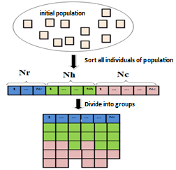
The chicken swarm can be divided into several groups as shown in Figure 2, each group containing: One dominant rooster, many hens and many chicks. It all depends on fitness values. The chickens with the best fitness are roosters, the chicks with the worst fitness are chicks, and the rest are hens.
Figure 2. Hierarchical system of the chicken swarm
2.2.2 Chicken movement
All the N virtual chickens, represented by their positions (Eq. (1)) at time step t, are looking for food in a D dimensional space. In this work, optimization problems are minimization. So the best chickens are those with minimal fitness values.
$x_{i, j}^{t}(i \in[1 \ldots N], j \in[1 \ldots D]$ (1)
Roosters’ movement. Roosters with better fitness are the priority for access to food than those with lower fitness values. For simplicity, roosters with better fitness may seek food in more places than roosters with worse fitness values. The movements of the roosters are:
$x_{i, j}^{t+1}=x_{i, j}^{t} *\left(1+\operatorname{randn}\left(0, \sigma^{2}\right)\right)$ (2)
$\sigma^{2}=\left\{\frac{1 \text { if } f_{i} \leq f_{k}}{e^{\frac{(f k-f i)}{|f i|+\varepsilon}}}\right\} k \in[1, N] k \neq i$ (3)
Movement of chickens. The chickens can follow the rooster of group to look for food. They stole good food found by other chickens although they would be suppressed by other chickens. The more dominant hens would benefit from competing for food than the less dominant ones.
$x_{i, j}^{t+1}=x_{i, j}^{t}+S 1 * \operatorname{rand}\left(x_{r 1, j}^{t}-x_{i, j}^{t+1}+S 2 *\right.$
rand $*\left(x_{r 2, i}^{t}-x_{i, i}^{t}\right)$ (4)
$S 1=e^{\left(\frac{(f k-f r 1)}{|f i|+\varepsilon}\right)}$ (5)
$S 2=e^{\left(f_{r 2}-f_{i}\right)}$ (6)
Chick movement. The chicks move around their mother in search of food. This is formulated below:
$x_{i, j}^{t+1}=x_{i, j}^{t}+F L^{*}\left(x_{m, j}^{t}-x_{i, j}^{t}\right)$ (7)
2.3 The main Steps of CSO algorithm
3.1 Problem formulation
The network's area of interest is a two-dimensional space with size L ⅹ L; we distribute a set of N sensors in this environment in a random way. We consider a specific number of (m > 0) sensors as anchors by determining their locations during the distribution process, either by placing them automatically or by providing them with a GPS device. The goal of the positioning process is to find the coordinates of the rest sensors labeled m + 1 ...N (N = n + m), those who fell into unknown places during the randomization process of distribution. Each sensor in the network is characterized by a similar transmission radius (R).
This positioning problem is optimizations problem in which we try to minimize a fitness function of (Eq. (8)), represent the difference between the calculated and estimated distances.
$f(x, y)=\frac{1}{M} * \sum_{i=1}^{M}\left(d_{i}-\hat{d}_{i}\right)^{2}$ (8)
$d_{i}$ Is the distance between the candidate position as a solution and the M anchors (where M≥3) directly connected to the sensor to be located. let (x, y) the coordinates of the target node, the distance between the target node and the anchor i (xi, yi) is calculated using the following Euclidean distance formula:
$d_{i}=\sqrt{\left(x-x_{i}\right)^{2}+\left(y-y_{i}\right)^{2}}$ (9)
$\hat{d}_{i}=d_{i}+d_{i} \times \frac{P_{n}}{100}$ it is the estimated distance between the true location of the target sensor and its directly related anchors; with pn it is the percentage noise in distance measurement by one of technologies RSSI, LQI, TOA...
3.2 Proposed localization algorithm
Identification of the initial population: randomly deploy in the area of interest Np (total number of individuals) chickens (specify Nr number of roosters, Nh number of chickens and Nc number of chicks). Figure 3 shows an applied example for the identification of each subgroup of chickens.
Calculate the fitness value: Calculate the fitness value of each individual in the population by the Eq. (8) then we determine best fitness values represents minimum value fbest and the position of the best individual (xbest, ybest).
Determine identity and subgroup of the chickens: In this step we will Identify the identity of the chickens (rooster, hen and chick), sorted all individuals of the population according to fitness, the Nr chickens with the minimum fitness values are designated as roosters, while Nc hens with maximum fitness values would be considered chicks and the rest are hens.
The swarm is divided into different groups, each rooster represents a group and considers as the leader of group, the hens randomly choose the group to live in and the chicks randomly choose hens as mothers and join the corresponding groups.
Figure 3. Determine identities and subgroups
Movement of chickens: Calculate using the Eqns. (2), (4) and (7) respectively the new coordinates of each individual of the chickens according to different identities. Calculate new fitness value, If the new fitness value is better than the current individual's fitness value updates the individual's position and fitness value Otherwise keep the old position.
NB: If the new coordinates transcend the L×L search space, then recalculate these positions.
Update global solution: If one of the new lower fitness values has the overall fitness value fbest, update the position (Xbest, Ybest) and the best fitness value fbest.
Provide the best overall solution: Repeat these processes of positioning, until you reach the maximum number of iterations, finally the final position of the unknown sensor is located.
The algorithm can estimate the locations of unknown sensors only if the number of anchors in the transmission range is greater or equal to 3. Improvements have been added to the proposed CSO algorithm for we can locate the greatest number of unknown sensors. Each sensor knowing enough 'anchors in its neighborhood, become an estimated anchor only if the error between its estimated position and its real position is less than threshold "(fitness value less than"). This information is then broadcast in the neighborhood which allows other sensors to locate.
Based on the previous steps, our proposal for locating sensors with unknown positions in wireless sensor networks is presented in detail in the flowchart of Figure 4.
Figure 4. Flowchart of the proposed approach
In order to prove the success of our proposal for the localization of nodes in WSN, we developed our application using MATLAB language version R2013a on Windows 8 Professional 32 bit, 2.00 GB RAM, and Intel (R) Core (TM) i3-2310 M CPU @ 2.10 GHz, 2.10GHz process.
In order to ensure a fair comparison, we did not just program our proposed approach, but added to this the programming of the algorithm proposed [16], which also based on CSO. In what follows, we will call our approach: Improved CSO and the approach proposed in 10 CSO.
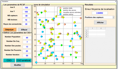
So that we can choose and modify any properties used, whether for the network or for intelligent systems, we have implemented a very rich interface is presented in following figure. In the Figure 5 the orange nodes represent the unknown sensors, the green nodes represent the anchors and the blue circles indicate the sensors located by CSO. Yellow circles indicate sensors considered as estimated anchors. We notice that the coordinates estimated by improved CSO are closer to the real coordinates than that estimated by classical CSO, and by our proposed method we can locate all the unknown sensors.
Figure 5. Interface of our simulation
4.1 Evaluation metric
To assess the accuracy of the localization methods used in this experiential study. The mean error should be calculated as the average of the differences between the actual positions and the positions estimated by these methods. The average error is calculated as follows:
$\operatorname{Error}_{A V G}=\left(\frac{\sum_{i}^{N} \sqrt{\left(X_{r}-X_{c}\right)^{2}+\left(Y_{r}-Y_{c}\right)^{2}}}{N}\right)$ (10)
where,
4.2 The influence of the parameters on precision of our approach
To know the effect of different parameters on the precision of the CSO algorithm, we carried out the following series of experiments in which we varied the desired parameter and we determined the other parameters to the values represented in the below table:
Table 1. Parameters used in experiments
|
Parameters |
value |
|
Area size |
100*100 m |
|
Number of sensors |
60 |
|
Number of anchors |
20 |
|
Transmission radius |
40 |
|
Population size |
40 |
|
Number of iterations |
50 |
In the first experiment we fix the different parameters on the values of Table 1 and we vary the number of sensors, the obtained results are presented in the Figure 6. This Figure clearly shows that the mean error value is increased with increasing number of sensors in the two CSO approaches and it can also be known that the mean error values of improved CSO is better than CSO.
Figure 6. Localization error Vs number of sensors
Figure 7. Localization error Vs number of anchors
Figure 8. Localization error Vs Population size
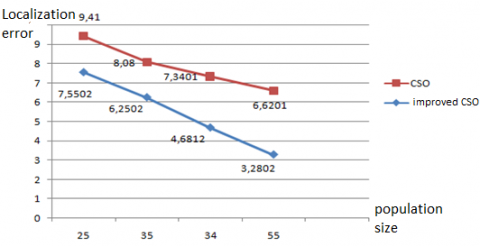
The results of the second experiment are shown in Figure 7. From these results, we conclude the value of the mean error decreases with increasing number of anchors for the two algorithms: CSO and improved CSO. Likewise, the location error relative to the population size will be calculated. From Figure 8, we see that the mean error decreases with increasing population size for the two algorithms: CSO and CSO improved, and we also see that the mean error of improved CSO is better than of CSO.
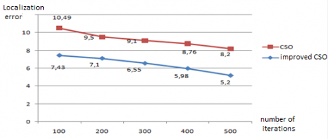
The graph below shows the localization error compared to the number of iterations. This Figure 9 clearly shows that the average error decreases with increasing number of iterations for the two algorithms: CSO and improved CSO.
Figure 9. Localization error Vs Number of iterations
4.3 Comparison of proposed approach with particle swarm optimization
In order to test and verify the performance of our proposition, we compare their performance with the PSO meta-heuristic of localization presented [9]; in this comparison we used the network configuration and algorithms parameters as follows:
Figure 10. Comparison between the three algorithms CSO, PSO and improved CSO
From Figure 10 which indicates the average error obtained by CSO, improved CSO and PSO when we change the number of anchors, it is clear that the value of the average error is decreased with the increase of the number of anchors, in the three algorithms. Note that the mean error values of CSO is greater than of PSO and improved CSO when the number of anchors equals 15, then becomes almost equal to PSO. And we can also see that the mean error of improved CSO is lower compared to the other two algorithms.
In this paper, we have proposed an improved CSO algorithm to enhance precision of localization in wireless sensor networks, based on the efficient meta-heuristic of chicken swarm optimization. In order to study the effect of network parameters and intelligent algorithms, we implement a rich interface of program in the simulation environment of MATLAB. In our simulation for ensure a fair comparison, we were not satisfied by programming our proposed approach, but we added to it another traditional CSO method of localization proposed [16]. The studies that we have carried out have demonstrated the clear effect of our proposed approach by changing the characteristics of the network and the number of chickens used, as well as its ability to improve the classical approach CSO; and the comparison results with PSO showing the superiority of proposed approach. Our approach is tested in static network and 2D area, and we hope to provide a version for mobile networks and 3D area of interest.
[1] Pal, A. (2010). Localization algorithms in wireless sensor networks: Current approaches and future challenges. Network Protocols and Algorithms, 2(1). https://doi.org/10.5296/npa.v2i1.279
[2] Niculescu, D., Nath, B. (2001). Ad hoc positioning system (aps). In Global telecommunications conference. GLOBECOM IEEE, 5: 2926-2931. http://dx.doi.org/10.1109/glocom.2001.965964
[3] Cho, H.H., Lee, R.H., Park, J.G. (2011). Adaptive parameter estimation method for wireless localization using RSSI measurements. Journal of Electrical Engineering and Technology, 6(6): 883-887. https://doi.org/10.5370/JEET.2011.6.6.883
[4] Moore, D., Leonard, J., Rus, D., Teller, S. (2004). Robust distributed network localization with noisy range measurements. In Second Int. Conf. on Embedded Networked Sensor Systems, pp. 50-61. https://doi.org/10.1145/1031495.1031502
[5] Siddique, N., Adeli, H. (2015). Nature inspired computing: An overview and some future directions. Cognitive Computation, 7(6): 706-714. https://doi.org/10.1007/s12559-015-9370-8
[6] Nan, G.F., Li, M.Q., Li, J. (2007). Estimation of node localization with a real-coded genetic algorithm in WSNs. 2007 International Conference on Machine Learning and Cybernetics, pp. 873-878. https://doi.org/10.1109/ICMLC.2007.4370265
[7] Kannan, A.A., Mao, G.Q., Vucetic, B. (2006). Simulated annealing based wireless sensor network localization. JCP, 1(2): 15-22. https://doi.org/10.4304/jcp.1.2.15-22
[8] Biswas, P., Ye, Y. (2004). Semi definite programming for ad hoc wireless sensor network localization. In Proceedings of the 3rd International Symposium on Information Processing in Sensor Networks, pp. 46-54. https://doi.org/10.1145/984622.984630
[9] Gopakumar, A., Jacob, L. (2008). Localization in wireless sensor networks using particle swarm optimization. 2008 IET International Conference on Wireless, Mobile and Multimedia Networks, pp. 227-230. https://doi.org/10.1007/s13369-017-2471-9
[10] Moussa, A., El-Sheimy, N. (2010). Localization of wireless sensor network using bees optimization algorithm. The 10th IEEE International Symposium on Signal Processing and Information Technology, pp. 478-481. https://doi.org/10.1109/ISSPIT.2010.5711760
[11] Cao, S., Wang, J.H., Gu, X.S. (2012). A Wireless Sensor Network Location Algorithm Based on Firefly Algorithm. Springer, Berlin, Heidelberg.
[12] Goyal, S., Patterh, M.S. (2014). Wireless sensor network localization based on cuckoo search algorithm. Wireless Personal Communications, 79(1): 223-234. https://doi.org/10.1007/s11277-014-1850-8
[13] Rabhi, S., Semcheddine, F. (2019). Localization in wireless sensor networks using DV-hop algorithm and fruit fly meta-heuristic. Advances in Modelling and Analysis B, 62(1): 18-23. https://doi.org/10.18280/ama_b.620103
[14] Rabhi, S., Semcheddine, F., Mbarek, N. (2021). An improved method for distributed localization in WSNs based on fruit fly optimization algorithm. Autom. Control Comput. Sci., 55(3): 286-296. https://doi.org/10.3103/S0146411621030081
[15] Meng, X., Liu, Y., Gao, X., Zhang, H. (2014). A New Bio-inspired Algorithm: Chicken Swarm Optimization. In: Tan Y., Shi Y., Coello C.A.C. (eds) Advances in Swarm Intelligence. ICSI 2014. Lecture Notes in Computer Science, vol 8794. Springer, Cham. https://doi.org/10.1007/978-3-319-11857-4_10
[16] Al Shayokh, M., Shin, S.Y. (2017). Bio inspired distributed WSN localization based on chicken swarm optimization. Wireless Pers Commun., 97: 5691-5706. https://doi.org/10.1007/s11277-017-4803-1