Iman Herwidiana Kartowisastro*![]() | Johanes Latupapua
| Johanes Latupapua![]()
© 2023 IIETA. This article is published by IIETA and is licensed under the CC BY 4.0 license (http://creativecommons.org/licenses/by/4.0/).
OPEN ACCESS
The rapid decline in wildlife animal diversity necessitates expedited evaluations of biodiversity and population dynamics. Accurate image recognition from camera traps is central to such assessments. This study investigates the impact of different optimisation techniques and hyperparameter configurations on the accuracy of wildlife animal classification. Specifically, the comparative effectiveness of the Adaptive Moment Estimation (Adam) and Root Mean Square Propagation (RMSProp) optimisation algorithms is examined. The influence of learning rates on these optimisation techniques is evaluated, while other hyperparameters are held constant. Convolutional Neural Networks (CNN) models, namely DenseNet-121, ResNet-50, and AlexNet, are utilised for this study. The investigation employs a dataset composed of 47,841 images sourced from the Serengeti Project Season 1 Snapshot in Tanzania. The images depict wild animals in diverse perspectives within their natural habitats, with some providing a complete view of the animal's body, while others do not. The dataset, characterised by an imbalanced distribution, is segregated into training, validation, and testing sets at proportions of 80%, 10%, and 10%, respectively. The results reveal that the application of the Adam optimisation technique yields the highest average accuracy of 80.66% with the ResNet-50 model. However, the DenseNet-121 model achieved an overall accuracy exceeding 95%. Notably, the ResNet-50 architecture, with learning rates of 0.1 and 0.01, encountered challenges during the training and validation of all images due to the complexity of the dataset. Irrespective of the optimisation technique employed, the most effective performance was observed with the ResNet-50 model, utilising the Adam optimiser and a learning rate of 0.001. The study proposes suitable learning rate values for training scenarios similar to the present investigation.
convolutional neural networks, wildlife animal classification, optimisation, Adam, RMSProp
The development of sensor technology in recent years has led to an increase in the use of data acquisition in animal ecology. However, there are still limitations when it comes to converting that data into relevant and important information. This may hinder the ability to get more benefits or capitalise on the large dataset obtained by those sensors, i.e., using machine learning techniques with knowledge. The decline in animal diversity affects not only genetics but also ecological and behavioural diversity [1]. A review of machine learning techniques to detect farm animal behaviour, e.g., lameness, grazing, and rumination, was conducted by Debauche et al. [2]. The review was based on sensors and algorithms used to detect each animal category.
As deep learning methods advance, object recognition through Convolutional Neural Networks (CNN) is steadily improving. The distinctive characteristics of various image-based objects have piqued the interest of researchers, driving them to develop learning techniques capable of achieving high accuracy. The CNN architecture continues to develop, starting with the creation of the AlexNet architecture, which was able to recognise objects in ImageNet by Krizhevsky et al. [3]. This research represented a major breakthrough in the advancement of deep learning. As a result, subsequent studies have given rise to novel architectural variations like Inception [4], ResNet [5], and various other architectures. Architecture types may affect the accuracy of the system, which also contributes to the research interests in devising new architectures.
In the field of insect detection, a study was conducted using Faster R-CNN with Inception V2 combined with an image processing approach to distinguish dengue mosquitoes. This approach was compared with R-FCN with Resnet-101 and SSD with MobileNet. As a classifier, in terms of accuracy, Faster R-CNN outpaced R-CCN and SSD for the test dataset [6].
In addition to the selection and design of CNN architecture, several elements, such as the size of the training and testing datasets, the hyperparameter value for training, normalisation, regularisation, and optimisation techniques, will determine the accuracy of the result. For micromachines, mathematical relationships were established among four hyperparameters: learning rate, batch size, dropout rate, and convolution kernel size. Additionally, a generalised multiparameter correlation model was formulated. Experimental results demonstrated that these relationships were vital to the neural network’s performance [5].
This study specifically discusses the learning rate configuration in gradient descent as a crucial hyperparameter for achieving high level of accuracy in the training process. The learning rate plays a crucial role in controlling the speed at which the model learns. Goodfellow et al. state that learning rate can be considered the most important hyperparameter [4]. Obtaining optimal learning rate values for a model with its corresponding datasets is not easy. The challenge lies in determining the appropriate hyperparameter values in the architecture. In order to speed up the optimisation process and have the right hyperparameter values, a technique was employed where lower-dimensional data was initially used and the dimensionality was progressively increased during the optimisation process [7].
This study discusses the application of Adaptive Moment Estimation (Adam) and RMSProp optimisation algorithms, which depend on the learning rate value, and their implementation on three CNN architectures. Recommendations are then provided based on the learning rate value of the Adam technique in animal classification. The comparison result from Adam is the optimisation of RMSProp to compare the value of achieved accuracy. Both optimisations are performed for the classification of animals in the wild, a domain where image characteristics exhibit significant variation. This subject has been the focus of extensive research in the past few years, attracting the attention of both biology and information technology researchers [8-11].
Animal pictures taken from various points of view, including the front view, provide numerous research challenges in achieving optimal accuracy. The camera trap technique involves capturing photographs of animals at various locations within a specific area over a designated time frame [12]. One of the major projects that collects datasets using camera traps and is publicly accessible is the Serengeti Snapshot, in which joint projects with animal photo collection and identification have been carried out, involving many communities [13], and data have been collected at a large geographic and temporal scale [14]. Another work on the Serengeti dataset was performed to identify, count, and describe the behaviours of wildlife animals with a deep Convolutional Neural Network approach. Five different architectures were tested: AlexNet, NiN, VGG, GoogLeNet, and ResNet. This effort concluded with ResNet having the best accuracy of 93.8% [15].
Similar projects in other countries have also been initiated in recent years. Among others, a study was conducted in Morocco to identify the presence and absence of insects, in this case, three mosquito species. Recursive feature elimination was carried out in combination with a cross-validation approach. Using the Scott Knott (SK) approach, some classification models were tested: 1. Gradient Boosting, 2. Random Forest, 3. XG Boost, 4. Logistic Regression, 5. KNN, and 6. Gaussian Naïve Bayes. The models were evaluated using performance measures including accuracy, Matthews Correlation Coefficient (MCC), and area under the ROC curve (AUC). The results indicated that the Gradient Boosting, Random Forest, and XGBoost algorithms were the most powerful models [16].
Based on the background information and explanation cited above, this paper compares Adaptive Moment Estimation (Adam) and RMSProp optimisation algorithms for wildlife animal classification using Convolutional Neural Networks. The aim is to answer the research question of how to increase the accuracy of wildlife animal classification. Hence, wildlife animal conservation initiatives can use this work to improve the camera trap result.
Both optimisation algorithms are known to respond well to changes in learning rate. The evaluation is carried out by incorporating these optimisation techniques into three architectures, DenseNet-121, ResNet-50, and AlexNet, to produce the highest possible accuracy.
This article is organised as follows: Section 2 outlines the research methodology, encompassing the literature review, optimisation techniques of Adaptive Moment Estimation (Adam) and Root Mean Square Propagation (RMSProp), research model, and dataset. Section 3 presents the results and analysis of the implementation of the optimisation technique mentioned above on three CNN architectures, namely Densenet-121, ResNet-50, and AlexNet. Finally, Section 4 presents the conclusion of this work.
2.1 Literature review in animal classification
The provision of public datasets of wildlife animals using camera traps has been conducted by several national park locations, where one of the largest datasets is Snapshot Serengeti, which currently comprises approximately 3.2 million images [13]. This dataset has been the object of research in subsequent studies. He et al. [14] presented their research for monitoring systems and the introduction of animals in the wild, from camera traps to data stored in the cloud. This system involves the public acting as a reviewer or photo provider.
Trnovszky et al. [17] conducted a study focused on the learning of five different animal types: wolves, foxes, bears, pigs, and deer. The CNN architecture used is similar to AlexNet. The study involved a comparison between CNN and several other techniques, namely Principal Component Analysis (PCA), Support Vector Machine (SVM), Local Binary Pattern Histograms (LBPH), and Linear Discriminant Analysis (LDA). The dataset used is publicly accessible, the Washington RGB-D Object Dataset, for testing and ImageNet as pre-training. The dataset consisted of 500 test images, with 100 images for each animal species captured from a frontal view only. The experimental results obtained by CNN resulted in a higher percentage of accuracy compared to the other four methods. For larger training set numbers without CNN, LBPH resulted in higher accuracy. However, the drawback is that the image was taken only from the front.
Nguyen et al. [18] carried out a study on the distribution of various species (imbalance class) in the wild, taking into consideration a larger number of classifications and diverse animal positions. Wildlife Spotter, a dataset consisting of 72,498 images encompassing 18 different animal types, was used in the study. Eighty percent of the images were used for training and twenty percent for validation. The positions of the animals were taken from multiple angles. The team compared three CNN architectures: VGG, Lite AlexNet, and ResNet-50. However, the best results of the experiments were obtained when the classes were still balanced, particularly for the six classes with the largest dataset. In this experiment, the VGG-16 architecture reached the highest accuracy of 95.88%. In training for the three highest classes of the dataset, the accuracy ranged from 89.16% to 90.4%.
In addition to the research conducted by Nguyen et al. [18], who used public datasets, Villa et al. [19] also conducted a study employing the Serengeti Snapshot dataset for 26 types of animals. They created a well-balanced class comprising 26,000 training images and 6240 test images. The dataset consists of four categories: imbalances, balances, foreground, and segmented. For animal recognition, Top-1 and Top-5 measurements were taken, proceeding from the lowest results to the maximum level of accuracy of imbalances, balances, foreground, and segmented. ResNet-101 attained the highest accuracy of 98.1% by combining four distinct dataset categories.
Zin et al. [20] conducted interesting research using Deep CNN (DCNN) that focused solely on cows. Forty-five forms of cows were sampled, and their data was captured in videos with a 30 fps frame rate. The image is captured from the live video and depicts either the full body or a partial view of the cows from the top or front perspective. The employed DCNN architecture consists of a single input layer, three convolutional pools, one fully connected layer, and one output layer. During the training phase, the identification of cows based on their full bodies achieved an accuracy score of 98.87%, while the test score reached 97.01%. In the case of partial body images, the accuracy score obtained was 86.8%.
Research with DCNN with an architecture similar to that of Zin et al. [20] was conducted by Chen et al. [10] with three convolutional and three max pooling. They conducted a comparison between DCNN and BoW (Bag of Visual Words) in conjunction with LDA (Linear Discriminant Analysis). The evaluation involved 14,346 training images and 9,530 testing images to identify 20 distinct classes of prominent wild animals found in North America. The DCNN results were still far below those of other studies, with a value of 38.315%.
Verma and Gupta [21] also conducted DCNN research using five convolutional pools and three fully connected layers, similar to AlexNet. The dataset was the same as that of Chen et al. [10]. The dataset contained 1,110 images, of which 90% were allocated for training while the 10% were reserved for testing. Additionally, SVM and KNN models were assessed alongside DCNN, with the accuracy of the DCNN model reaching 91%.
Tabak et al. [22] used more than 3 million images from five US states, Canada, and the Serengeti Snapshot (Tanzania) as their dataset. This classification used the ResNet-18 architecture with a 16 GB RAM Macintosh laptop. The training accuracy results for the US dataset attained 98%, while the validation results from Canada and Tanzania were 82% and 94%, respectively. Another interesting study involved generalisation by testing images from locations where training had never been done. Schneider et al. [23] conducted this study using 47,000 datasets from five locations with five architectures.
Several researchers have conducted studies on the application of animal detection and monitoring, both as standalone systems, such as for livestock monitoring, and integrated with other technologies. Yousif et al. [24], Guzhva et al. [25], Hansen et al. [26], Rivas et al. [27], and Schneider et al. [28] have contributed to this field of research.
Gradient class activation procedures have been studied aimed at extracting the most salient pixels within the final convolutional layer [29]. The dataset was comprised of 20 classes of wild animals from Africa.
2.2 Method development
This research analyses the classification of animal images in three of CNN’s most recent architectures, namely Densenet-121, ResNet-50, and AlexNet. A comparison using Adaptive Moment Estimation (Adam) and Root Mean Square Propagation (RMSProp) as optimisation techniques was executed in the training stage. With Adam, the advantages of training processes are faster and more stable training processes to achieve the highest accuracy value [30]. One parameter that is within the scope of this research is the learning rate, with the notation LR. Both optimisations depend on the learning rate value, so the effect of changes to the accuracy value will be known. Classification is conducted using an image dataset that is based on images from camera traps with different lighting levels and animal positions, where photos are taken during the day and night. All these images represent real conditions in a wildlife conservation park. The dataset used in this research is sourced from the Serengeti Project Snapshot season 1 in Tanzania, and sufficient light conditions were taken. Figure 1 illustrates the research model employed in this study.
Figure 1. Research model
The dataset falls into the imbalance class and is divided into three folders for training, validation, and testing, with a proportion of 80%, 10%, and 10%, respectively. There are no overlapping images between those three folders. During the preprocessing stage, not all datasets are used by manually excluding images of lower quality, such as those that are too dark or black and white. Consequently, 46,841 images were selected, representing 11 different animal classes.
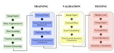
Figure 2. Implementation flow
The design was implemented on FloydHub.com, a frequently utilised cloud-based deep learning platform. This study used two types of Nvidia products: the Tesla V100 RAM (16 GB), and the Tesla K80 RAM (16 GB). The authors wrote the program code using the Anaconda platform, Jupyter Notebook, the PyTorch framework, and Python 3.7. Figure 2 shows how the model was implemented in detail, from taking input to computing accuracy.
The system is designed to accept image input. In preprocessing, animal images are placed in their class name folders as subfolders of the training, validation, and testing folders. In the process of training, validation, and testing, iterations are taken randomly. The file size in the input is changed to 224 x 224 according to the input sizes of AlexNet, Resnet-50, and DenseNet-121. A series of transformations and data augmentation techniques are applied to each image in the training, validation, and testing folders. These include random horizontal flips, resize crops, centre crops, and normalisation. The DataLoader is then used to load the customised images into each respective folder. During the initial step, the training DataLoader is activated to load and process the training images.
In this research, the authors conducted transfer learning by applying a pretrained model to the ImageNet dataset, which has 1000 classes of goods, flora, and fauna. Prior to training with the animal dataset, the machine downloads and updates the parameters, allowing the model to be available from the outset. With this, the engine already has a model at the beginning. Once the pretraining process is completed, feature extracting is performed. This extraction process solely considers gradients without the initial parameters from the pretrained outcomes, and adjusts the final output layer based on the quantity of classes and architectural variations.
During the training stage, a forward pass is executed at the beginning, and then a backpropagation is run while calculating a loss. When running the optimizer step, the parameter update is performed. This process of forward pass, backpropagation, and parameter update is repeated for a specified number of training sessions. Upon completion of the training, total loss and accuracy are calculated. For validation and testing, it is almost the same order as the forward pass but without backpropagation. Loss and accuracy are accumulated from each process to become the final loss and accuracy.
The results of the calculation of accuracy in training and testing are displayed graphically, so the movement between using RMSProp and Adam can be clearly seen. Accuracy is calculated with Top 1 by looking at average accuracy and highest accuracy in the testing stage.
2.3 Dataset
Serengeti National Park, located in Tanzania, Africa, is one of the sites listed by UNESCO as a world heritage site. It comprises 1.5 million hectares of savannah and is home to the largest remaining unaltered animal migration in the world. The dataset of the Serengeti Snapshot as a whole is extensive, containing approximately 3.2 million images from 11 seasons. However, only about 20% contain animal objects. In this research, 46,841 images were manually selected [31]. The total number of classes in this study was 11, which exhibited an imbalance in class distribution.
Many pictures taken depict animals in their natural environment. This creates another challenge in the research, as it not only gives pictures taken from various angles but also gives pictures that only show part of the animal’s body.
Dataset condition
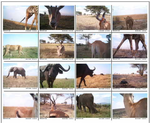
The dataset used was taken from Project Snapshot Serengeti season 1. Overall, the dataset consists of approximately 75% of images without animals, and it encompasses 47 animal classes. In preprocessing before the program is executed, image selection with three criteria is done: separating pictures of animals or without animals; taking pictures in the morning, afternoon, and evening only; and selecting classes with not less than 1000 pictures. From these three criteria, details are obtained with 46,841 images [31]. These images capture animals from different viewpoints, including front, side, and rear views, as shown in Figure 3. Furthermore, the dataset includes images depicting both full-body and partial-body views of animals and images featuring smaller animals within the frame. This is enough to describe the real issues caused by an imbalanced dataset when it is used to conduct research.
Figure 3. Animal in Snapshot Serengeti with different view angles comprising a combination of full pictures and partial pictures
Several previous studies have been described in Section 2.1, and some of them used a dataset of more than 1 million images. The resulting accuracy reaches> 90%. From the results obtained by the author, the accuracy of the classification of animals in the wild with several kinds of positions can reach> 90% with a number of datasets of tens of thousands. The author did not discuss the relationship between lighting levels and accuracy results. The principle is that as long as there is sufficient light, the image can be used in classification with CNN.
2.4 Adaptive moment estimation (Adam) and Root Mean Square Propagation (RMSProp)
Optimisation algorithms that are based on gradient descent are selected in this work due to their good convergence in non-convex problems, in which Adam and RMSProp fall into this category. Hence, the research specifically focuses on utilising these optimisation techniques, Adam and RMSProp, and comparing their accuracy results. Adam is a stochastic optimisation requiring only first-order gradients with low memory usage [27]. Adam brings together the benefits of AdaGrad, which demonstrates effectiveness for sparse gradients, and RMSProp, which performs effectively in both online and non-stationary scenarios. Both of these techniques maintain the learning rate. Previously, Stochastic Gradient Descent (SGD) was a popular optimisation technique used in machine learning.
Intuitively, the learning rate (step size) is not constant depending on the current gradient value; it is high when it is far from the minimum value and low when it is close to the minimum value. AdaGrad solves the problem in SGD, which applies η that was adaptive to the default value of 0.01. The AdaGrad formula is as follows:
$\theta_{t+1}=\theta_t-\frac{\eta}{\sqrt{G_t+\epsilon}} g_t$ (1)
where:
$\theta$ = weight parameter value
$G$ = total squares of the gradient with respect to all parameters of $\theta$.
$\varepsilon$ = a small positive number.
$g$ = moving average of squared gradient
$\eta$ = learning rate
$t$ = a particular time instant
This changes the value of η in the iteration of t for each parameter θibased on the gradient value obtained previously for the parameter θi. The disadvantage of this algorithm is that the previous gradient value in the denominator keeps growing, which will cause a lower learning rate and hence stop the training process.
The Root Mean Square Propagation (RMSProp) technique tries to avoid the condition of stop learning occurring in AdaGrad by calculating the moving average of the root mean square over the gradient using the following formula:
$\mathrm{E}\left[\Delta \theta^2\right]_{\mathrm{t}}=\gamma \mathrm{E}\left[\Delta \theta^2\right]_{t-1}+(1-\gamma) \Delta \theta_{\mathrm{t}}^2$ (2)
The root mean squared error value of the corresponding parameter update is represented by
$\operatorname{RMS}[\Delta \theta]_{\mathrm{t}}=\sqrt{\mathrm{E}\left[\Delta \theta^2\right]_{\mathrm{t}}+\varepsilon}$ (3)
$\mathrm{E}\left[\mathrm{g}^2\right]_{\mathrm{t}}=0.9 \mathrm{E}\left[\mathrm{g}^2\right]_{\mathrm{t}-1}+0.1 \mathrm{~g}_{\mathrm{t}}^2$ (4)
$\Delta \theta_t=-\frac{\eta}{\sqrt{E\left[g^2\right]_t+\varepsilon}} g_t$ (5)
where, γ denotes a constant. Krizhevsky et al. [3] recommend γ = 0.9. The result of this RMS formula is the value for the exact same rule update as AdaGrad. The combination of these two functions allows RMSProp to change learning rates adaptively while preventing them from becoming too small.
Adam is an optimisation algorithm like RMSProp, which has momentum. Adam stores the RMS and gradient averages from previous iterations [26]. These two values are called first momentum (mt) and second momentum (vt). The formula for first-order momentum (mt) with decay rate β1 = 0.9 and second-order momentum (vt) with decay rate β2 = 0.999 is as follows:
$m_t=\beta_1 m_{t-1}+\left(1-\beta_1\right) g_t$ (6)
$v_t=\beta_2 v_{t-1}+\left(1-\beta_2\right) g_t^2$ (7)
where, mt and vt are the values of moment (1st moment) and variance (2nd moment), respectively.
Furthermore, the results of the formula mentioned above are further refined through the bias correction process so that the corrected first-order momentum and second-order momentum are
$\widehat{\mathrm{m}}_{\mathrm{t}}=\frac{\mathrm{m}_{\mathrm{t}}}{1-\beta_1^{\mathrm{t}}}$ (8)
$\hat{v}_t=\frac{v_t}{1-\beta_2^t}$ (9)
The final result is,
$\theta_{\mathrm{t}+1}=\theta_{\mathrm{t}}-\frac{\eta}{\sqrt{\hat{\mathrm{v}}_{\mathrm{t}}}+\varepsilon} \widehat{\mathrm{m}}_{\mathrm{t}}$ (10)
Testing was conducted by measuring the accuracy achieved from each change in learning rate by DenseNet-121, ResNet-50, and AlexNet, where everything is done with Adam and RMSProp. Some parameters are kept consistent, namely, batch size = 32, epoch = 30, and loss function using cross-entropy loss due to the classification for multiclass. The author ran transfer learning with feature extracting by DenseNet-121, ResNet-50, and AlexNet. The learning rate value tested starts at 0.1 and decreases to one-tenth of the previous values, which are 0.1, 0.01, and 0.001.
This research conducts transfer learning before training to avoid building architecture and training from scratch. The advantage is that one of the current transfer learning models, besides finetuning, is feature extracting. In the feature extraction, it is pretrained on the ImageNet dataset and followed by the last layer modification.
3.1 RMSProp implementation
Table 1 shows the average value of testing accuracy from a single test execution with 140 samples. The accuracy of AlexNet increases as the learning rate decreases. ResNet and DenseNet, however, stagnate or drop at learning rates 0.1 and 0.01 even though DenseNet was above 70% in all three learning rate values. ResNet has a residual learning property, which results in reduced training time and increased sensitivity to changes in learning rate. This is evident in the results, in which for a learning rate of 0.001, ResNet has the highest increase from the previous learning rate of 0.01.
Table 1. Mean accuracy result using RMSProp
|
Architecture |
Learning Rate (η) |
||
|
0.1 |
0.01 |
0.001 |
|
|
AlexNet |
73.55% |
72.95% |
78.76% |
|
ResNet-50 |
53.42% |
53.42% |
77.44% |
|
DenseNet-121 |
72.03% |
71.56% |
78.91% |
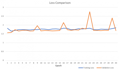
In cases where the accuracy remains consistently below 60%, one of the results of ResNet-50 is taken and processed in the form of a comparison graph of training loss and validation loss for a learning rate of 0.01, as depicted in Figure 4.
Based on Figure 4, there is a noticeable trend where the training loss and validation loss exhibit more stability and remain relatively constant, particularly in the case of the training loss. This condition means that ResNet-50 architectures with learning rates of 0.1 and 0.01 cannot conduct training properly on all training images and validation due to the complexity of existing datasets. The calculation formula for the RMSProp algorithm is as follows: θt: = θt - 1 - αgt / (√ nt + ε). When α (learning rate) gets smaller, θt value will be even greater. Conversely, with a greater learning rate, θt gets smaller. It means that the momentum θt does not reach the optimum value of accuracy. This can explain the condition of ResNet-50, which tends to be constant at around 50% but increases at a learning rate of 0.001.
Figure 4. Loss comparison in ResNet-50 using a learning rate of 0.1
Table 2. Highest accuracy result using RMSProp
|
Architecture |
Learning Rate (η) |
||
|
0.1 |
0.01 |
0.001 |
|
|
AlexNet |
87.50% |
90.62% |
93.75% |
|
ResNet-50 |
78.12% |
75.00% |
96.88% |
|
DenseNet-121 |
90.62% |
96.88% |
96.88% |
From Table 2, using RMSProp can achieve the highest accuracy for all three architectures with values> 93% at a learning rate of 0.001.
3.2 Adam implementation
Similar to RMSProp, Adam’s accuracy in three architectures increases as the learning rate decreases, as shown in Table 3. ResNet-50 accuracy, however, is still less than 60%, with learning rates of 0.1 and 0.01. The conditions are comparable to using RMSProp, where ResNet-50 cannot properly train all training images and validate its performance with the complexity of the existing dataset.
Table 3. Mean accuracy result using Adam
|
Architecture |
Learning Rate (η) |
||
|
0.1 |
0.01 |
0.001 |
|
|
AlexNet |
73.89% |
75.41% |
76.03% |
|
ResNet-50 |
53.42% |
58.40% |
80.66% |
|
DenseNet121 |
69.64% |
75.06% |
79.87% |
Table 4. Highest Accuracy result using Adam
|
Architecture |
Learning Rate (η) |
||
|
0.1 |
0.01 |
0.001 |
|
|
AlexNet |
93.75% |
90.62% |
90.62% |
|
ResNet-50 |
75.00% |
84.38% |
96.88% |
|
DenseNet-121 |
90.62% |
93.75% |
100.00% |
Table 4 shows that using Adam, the highest accuracy can be achieved by all three architectures with values >90% at a learning rate of 0.001. Notably, DenseNet achieves exceptional accuracy, with some samples reaching 100% accuracy out of the 140 tested.
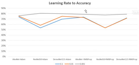
Subsequently, combining the results of Table 1 and Table 3 will produce a graph, represented in Figure 5.
Figure 5. Learning rate to accuracy
The maximum accuracy attained in this experiment was observed at a learning rate value of 0.001, indicating that the learning process occurred in more detail. There is a tendency for accuracy to increase with learning rates below 0.001. This condition, however, was not examined in this work. Figure 5 also shows that ResNet-50 is effective with a small learning rate, i.e., 0.001, when it outperforms AlexNet and DenseNet either with Adam or RMSProp.
In general, the accuracy of Adam is higher than that of RMSProp. Nevertheless, RMSProp remains a viable option because the average testing accuracy reaches more than 70%, and even the highest accuracy can reach more than 90%, as shown in Table 2.
Current work does not give enough opportunity to take advantage of the residual learning inherent in certain architectures. As a result, there is ample room for future research and exploration in this area.
This paper evaluated the performance of the CNN architectures DenseNet-121, ResNet-50, and AlexNet using Adaptive Moment Estimation (Adam) and RMSProp optimisation algorithms. While both optimisation techniques are based on the gradient descent approach, Adam outperforms RMSProp in terms of accuracy. This is attributed to the second-moment factor inherent in the Adam method.
The increase in accuracy value is dependent on the training process and the data used with the same architecture and hyperparameter. The maximum accuracy was attained with a learning rate value of 0.001, while the highest average accuracy was obtained with a value of 80.6% from the dataset of wildlife animal classification by DenseNet-121 architecture. The impact of hyperparameter, i.e., learning rate, on ResNet-50 architecture has different results than AlexNet and DenseNet-121. Hence, analysis with respect to learning rate is important in designing a Convolutional Neural Network. Furthermore, there is a tendency for accuracy to increase when the learning rate is <0.001. This finding opens opportunities for future research work as well as considering residual learning properties.
To conclude, the motivation, results, and discussion on optimisation algorithms, learning rates, and CNN architectures in this work can contribute to and enrich further research not only in CNN and optimisation subjects but also in a broader area, such as ecological and wildlife animal fields.
The authors would like to thank Bina Nusantara University for granting a professorship research program opportunity. This paper would probably not have been possible without such an opportunity.
[1] Tuia, D., Kellenberger, B., Beery, S., et al. (2022). Perspectives in machine learning for wildlife Conservation. Nature Communications, 13(1): 792. https://doi.org/10.1038/s41467-022-27980-y
[2] Debauche, O., Elmoulat, M., Mahmoudi, S., Bindelle, J., Lebeau, F. (2021). Farm animals’ behaviors and welfare analysis with AI algorithms: A review. Revue d'Intelligence Artificielle, 35(3): 243-253. https://doi.org/10.18280/ria.350308
[3] Krizhevsky, A., Sutskever, I., Hinton, G.E. (2012). Imagenet classification with deep convolutional neural networks. Advances in Neural Information Processing Systems, 25: 1097-1105.
[4] Szegedy, C., Ioffe, S., Vanhoucke, V., Alemi, A. (2017). Inception-v4, inception-resnet and the impact of residual connections on learning. In Proceedings of the AAAI Conference on Artificial Intelligence, 2017: 4278-4284.
[5] He, K., Zhang, X., Ren, S., Sun, J. (2016). Deep residual learning for image recognition. In Proceedings of the IEEE Conference on Computer Vision and Pattern Recognition, pp. 770-778. https://doi.org/10.1109/CVPR.2016.90
[6] Siddiqua, R., Rahman, S., Uddin, J. (2021). A deep learning-based dengue mosquito detection method using faster R-CNN and image processing techniques. Annals of Emerging Technologies in Computing (AETiC), 5(3): 11-23. https://doi.org/10.33166/AETiC.2021.03.002
[7] Shen, M., Yang, J., Li, S., Zhang, A., Bai, Q. (2021). Nonlinear hyperparameter optimization of a neural network in image processing for micromachines. Micromachines, 12(12): 1504. https://doi.org/10.3390/mi12121504
[8] Goodfellow, I., Bengio, Y., Courville, A. (2016). Deep learning. MIT Press. https://www.deeplearningbook.org/.
[9] Hinz, T., Navarro-Guerrero, N., Magg, S., Wermter, S. (2018). Speeding up the hyperparameter optimization of deep convolutional neural networks. International Journal of Computational Intelligence and Applications, 17(2): 1850008. https://doi.org/10.1142/S1469026818500086
[10] Chen, G., Han, T.X., He, Z., Kays, R., Forrester, T. (2014). Deep convolutional neural network based species recognition for wild animal monitoring. In 2014 IEEE International Conference on Image Processing (ICIP) Paris, France, pp. 858-862. https://doi.org/10.1109/ICIP.2014.7025172
[11] Willi, M., Pitman, R.T., Cardoso, A.W., Locke, C.M., Swanson, A., Boyer, A., Veldthuis, M., Fortson, L. (2019). Identifying animal species in camera trap images using deep learning and citizen science. Methods in Ecology and Evolution, 10(1): 80-91. https://doi.org/10.1111/2041-210X.13099
[12] Green, S.E., Rees, J.P., Stephens, P.A., Hill, R.A., Giordano, A.J. (2020). Innovations in camera trapping technology and approaches: The integration of citizen science and artificial intelligence. Animals, 10(1): 132. https://doi.org/10.3390/ani10010132
[13] Swanson, A., Kosmala, M., Lintott, C., Simpson, R., Smith, A., Packer, C. (2015). Snapshot Serengeti, high-frequency annotated camera trap images of 40 mammalian species in an African savanna. Scientific Data, 2(1): 1-14. https://doi.org/10.1038/sdata.2015.26
[14] He, Z., Kays, R., Zhang, Z., Ning, G., Huang, C., Han, T.X., Millspaugh, J., Forrester, T., McShea, W. (2016). Visual informatics tools for supporting large-scale collaborative wildlife monitoring with citizen scientists. IEEE Circuits and Systems Magazine, 16(1): 73-86. https://doi.org/10.1109/MCAS.2015.2510200
[15] Norouzzadeh, M.S., Nguyen, A., Kosmala, M., Swanson, A., Palmer, M.S., Packer, C., Clune, J. (2018). Automatically identifying, counting, and describing wild animals in camera-trap images with deep learning. Proceedings of the National Academy of Sciences, 115(25): E5716-E5725. https://doi.org/10.1073/pnas.1719367115
[16] Douider, M., Amrani, I., Balenghien, T., Bennouna, A., Abik, M. (2022). Impact of recursive feature elimination with cross-validation in modeling the spatial distribution of three mosquito species in Morocco. Revue d’Intelligence Artificielle 36(6): 855-862. https://doi.org/10.18280/ria.360605
[17] Trnovszky, T., Kamencay, P., Orjesek, R., Benco, M., Sykora, P. (2017). Animal recognition system based on convolutional neural network. Advances in Electrical and Electronic Engineering, 15(3): 517-525. https://doi.org/10.15598/aeee.v15i3.2202
[18] Nguyen, H., Maclagan, S.J., Nguyen, T.D., Nguyen, T., Flemons, P., Andrews, K., Ritchie, E.G., Phung, D. (2017). Animal recognition and identification with deep convolutional neural networks for automated wildlife monitoring. In 2017 IEEE International Conference on Data Science and Advanced Analytics (DSAA) Tokyo, Japan, pp. 40-49. https://doi.org/10.1109/DSAA.2017.31
[19] Villa, A.G., Salazar, A., Vargas, F. (2017). Towards automatic wild animal monitoring: Identification of animal species in camera-trap images using very deep convolutional neural networks. Ecological Informatics, 41: 24-32. https://doi.org/10.1016/j.ecoinf.2017.07.004
[20] Zin, T.T., Phyo, C.N., Tin, P., Hama, H., Kobayashi, I. (2018). Image technology based cow identification system using deep learning. In Proceedings of the International Multiconference of Engineers and Computer Scientists, 1: 236-247.
[21] Verma, G.K., Gupta, P. (2018). Wild animal detection from highly cluttered images using deep convolutional neural network. International Journal of Computational Intelligence and Applications, 17(4): 1850021. https://doi.org/10.1142/S1469026818500219
[22] Tabak, M.A., Norouzzadeh, M.S., Wolfson, D. W., et al. (2019). Machine learning to classify animal species in camera trap images: Applications in ecology. Methods in Ecology and Evolution, 10(4): 585-590. https://doi.org/10.1101/346809
[23] Schneider, S., Greenberg, S., Taylor, G.W., Kremer, S.C. (2020). Three critical factors affecting automated image species recognition performance for camera traps. Ecology and Evolution, 10(7): 3503-3517. https://doi.org/10.1002/ece3.6147
[24] Yousif, H., Yuan, J., Kays, R., He, Z. (2019). Animal Scanner: Software for classifying humans, animals, and empty frames in camera trap images. Ecology and Evolution, 9(4): 1578-1589. https://doi.org/10.1002/ece3.4747
[25] Guzhva, O., Ardo, H., Nilsson, M., Herlin, A., Tufvesson, L. (2018). Now you see me: Convolutional neural network based on tracker for dairy cows. Frontiers in Robotics and AI, 5: 107. https://doi.org/10.3389/frobt.2018.00107
[26] Hansen, M.F., Smith, M.L., Smith, L.N., Salter, M.G., Baxter, E.M., Farish, M., Grieve, B. (2018). Towards on-farm pig face recognition using convolutional neural networks. Computers in Industry, 98: 145-152. https://doi.org/10.1016/j.compind.2018.02.016
[27] Rivas, A., Chamoso, P., González-Briones, A., Corchado, J.M. (2018). Detection of cattle using drones and convolutional neural networks. Sensors, 18(7): 2048. https://doi.org/10.3390/s18072048
[28] Schneider, S., Taylor, G.W., Kremer, S. (2018). Deep learning object detection methods for ecological camera trap data. In 2018 15th Conference on Computer and Robot Vision (CRV) Toronto, ON, Canada, pp. 321-328. https://doi.org/10.1109/CRV.2018.00052
[29] Miao, Z., Gaynor, K.M., Wang, J., Liu, Z., Muellerklein, O., Norouzzadeh, M.S., Mclnturff, A., Bowie, R.C.K., Nathan, R., Yu, S.X., Getz, W.M. (2019). Insights and approaches using deep learning to classify wildlife. Scientific Reports, 9(1): 8137.
[30] Kingma, D.P., Ba, J. (2014). Adam: A method for stochastic optimization. arXiv preprint arXiv:1412.6980.
[31] Latupapua, J.M.B., Kartowisastro, I.H. (2020) Performance evaluation of convolutional neural networks and optimizers on wildlife animal classification. International Journal of Advanced Trends in Computer Science and Engineering, 9(5): 8686-8694. https://doi.org/10.30534/ijatcse/2020/256952020