Weixiang Jiang
© 2020 IIETA. This article is published by IIETA and is licensed under the CC BY 4.0 license (http://creativecommons.org/licenses/by/4.0/).
OPEN ACCESS
Most of the existing classification algorithms perform poorly facing big data samples. To solve the problem, this paper puts forward a novel classification algorithm based on backpropagation neural network (BPNN). Firstly, the original data were normalized to the same order of magnitude. The normalization improves the consistency of the input data, facilitating the classification. Next, the least mean square (LMS) algorithm and the BPNN were integrated into a novel batch learning BP algorithm. Finally, several experiments were carried out, revealing that our algorithm outshined the traditional BP algorithm in the classification accuracy. This research provides a good reference for the accurate classification of big data samples.
classification algorithm, big data, backpropagation neural network (BPNN), batch learning, multi-layer perceptron (MLP)
Classification is an important and common task in many branches of data mining. Data classification aims to abstract meaningful models from original data, making it possible to predict future trends. In general, this aim is realized in two stages: the learning stage and the classification stage. The former mainly sets up a classifier that describes the training set properly, while the latter relies on the classifier to make predictions [1, 2].
To obtain a proper classifier, the learning stage often adopts a classification algorithm to analyze the original dataset, and randomly extract the training set from the dataset. The extracted training set usually includes sample data tuples, and their class labels. This learning stage is also called supervised learning, as the class labels of tuples in the training set are already known. The learning process can be essentially described by a function y = f(x), which represents the correspondence between tuples and their class labels. This function helps to predict the class labels of tuples in the test set.
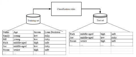
In the classification stage, the accuracy of the classifier is verified on the test set, which consists of test tuples and their class labels. The class labels predicted by the classifier are compared with the actual class labels, revealing the accuracy of the classifier and the prediction accuracy of the classification algorithm. Figure 1 explains the entire classification procedure with an example, in which multiple consumers are classified based on age, income, and credit risk.
The common classification algorithms are mainly based on statistical method [3, 4], decision tree (DT) [5-7], and the neural network (NN) [8, 9]. In addition, some classification algorithms draw the merits from the k-nearest neighbor (k-NN) algorithm [10, 11], support vector machine (SVM) [12] and so on.
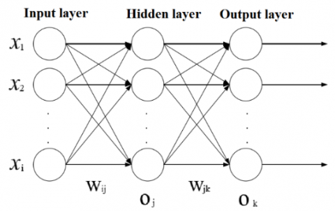
The NN is a complex interconnected system, whose nature and function depend heavily on the highly variable connection mode between neurons. Most of the NNs are feedforward neural networks (FNNs) [13] (Figure 2).
Figure 1. The entire classification procedure
Figure 2. The structure of a typical FNN
This paper mainly improves the backpropagation (BP) algorithm for the classification of big data samples. Firstly, the input data were normalized into the range of [0, 10], such that all input samples belong to the same order of magnitude. Then, the traditional BP algorithm was improved based on the backpropagation neural network (BPNN), a typical multi-layer perceptron (MLP), the least mean square (LMS) algorithm, and a self-designed momentum factor. To the best of our knowledge, this is the first attempt to fully integrate these techniques into the classifier of big data samples.
As mentioned above, the connection mode between neurons directly bears on the nature and function of the NN. In machine learning (ML), the perceptron is an NN for supervised learning of binary classifiers. Based on the eigenvector of an instance, the perceptron can output the class of the instance.
The perceptron is either single-layer perceptron (SLP) or MLP. The SLP is the simplest form of the FNN, which contains no hidden layer. By contrast, the MLP involves at least one hidden layer. Here, only the MLP is discussed in the light of our objective. The BPNN is a typical MLP.
As shown in Figure 3, the MLP encompasses several fully connected layers of neurons. The input x of the MLP has n features from the data pairs (x, d) in the training set. The neurons in the input layer are connected with the J neurons in the hidden layer via the weight vector V, while the J neurons in the hidden layer are connected with the K neurons in the output layer via weight vector W. Obviously, the input value has a direct impact on the output of the MLP. This makes preprocessing of input data a necessity.
In the same dataset, the sample values may vary greatly. Sometimes, a sample value might be hundred or even thousands of times that of another one. Hence, the input samples of the MLP could belong to vastly different orders of magnitude. Here, the input data are normalized to ensure that all sample values have the same order of magnitude.
To promote the prediction effect, the input of the MLP should cover a large proportion of training samples. Otherwise, the trained MLP will have a poor prediction effect. The preprocessing of input data needs to solve a key problem: speeding up the MLP training, while avoiding the impact of uneven distribution of training samples on the network.
2.1 Algorithm design
Since the original data are usually unordered, the training set might contain data scattering in a wide value range. In some cases, the data differ markedly in the order of magnitude. If the training set is directly applied, the training speed will be slowed down, and the trained MLP will have a poor accuracy. These negative impacts are explained as follows:
The MLP training mainly modifies the connection weights based on global error. These weights need to be modified in a long time, such that the connection weights could meet the requirements of both large samples and small samples. The time-consuming modification drags down the training speed. Meanwhile, the training samples are distributed unevenly on each scale. After training, the modified connection weights cannot reflect the features of most training samples. As a result, the input data must be normalized to facilitate the data prediction.
Numerical normalization is a popular way to minimize the scale difference between data. However, the numerically normalized data will still have a huge difference in magnitude. This means numerical normalization alone cannot satisfy the demand for the MLP. Thus, this paper normalizes the input data into the range of [0, 10] in two steps:
Firstly, the eigenvalue of each data was extracted. Considering their scale difference, the eigenvalues were converted into the same order of magnitude between 0 and 10. The interval of [0, 10] was selected, marking the first time that a specific range is defined for data preprocessing [14, 15]. Secondly, the extracted eigenvalues were multiplied by 10n, where the value of n depends on the specific dataset.
After the normalization, the classification algorithm could be obtained. The data in the test set should also be converted into the same scale, laying the basis for data prediction. Finally, the prediction results should be converted inversely to be compared with the original data.
The above input normalization method can be defined as:
Suppose training set T consists of P samples, each of which has M features and N outputs. Let Xi and Yi be input and output vectors, respectively, and Zi be the converted value. The value of Zi falls between 0 and 10. These vectors can be defined as follows: Xi=(Xi1, Xi2,…,XiM), Yi=(Yi1, Yi2,…,YiN), Zi=XiP*10n, and $Z_{i P} \in[0,10]$, where i=1,2,…P.
Figure 3. The structure of an MLP
2.2 Experimental verification
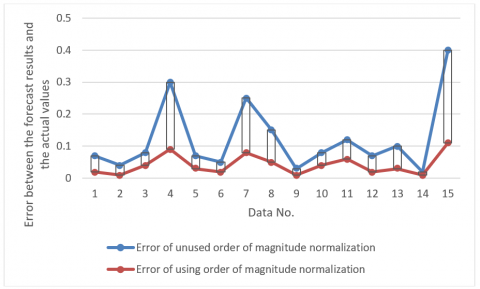
To verify the effectiveness of the above method, the BPNN algorithm was adopted to train a classifier with data on mineral composition, which was then used to predict the burning effect of different minerals. The test set contains 15 samples. Two parallel experiments were carried out. One of them directly uses the original data, which differ in the order of magnitude; the other uses the data normalized by the above method. Table 1 and Figure 4 both compare the errors between the prediction results and the actual values of the two experiments. It can be seen that the prediction was more accurate after the input data were normalized by the above method. Therefore, the above input normalization method can indeed improve the classification accuracy.
Table 1. Comparison between two experiments in prediction error
|
Sample number |
Prediction error of using normalized data |
Prediction error of using original data |
|
1 |
0.02 |
0.07 |
|
2 |
0.01 |
0.04 |
|
3 |
0.04 |
0.08 |
|
4 |
0.09 |
0.30 |
|
5 |
0.03 |
0.07 |
|
6 |
0.02 |
0.05 |
|
7 |
0.08 |
0.25 |
|
8 |
0.05 |
0.15 |
|
9 |
0.01 |
0.03 |
|
10 |
0.04 |
0.08 |
|
11 |
0.06 |
0.12 |
|
12 |
0.02 |
0.07 |
|
13 |
0.03 |
0.10 |
|
14 |
0.01 |
0.02 |
|
15 |
0.11 |
0.40 |
Figure 4. Comparison between two experiments in prediction error
This subsection designs a novel batch learning classification algorithm based on the MLS, an adaptive learning algorithm [16], and the BPNN.
3.1 Algorithm design
In the LMS, a cost function $\tau(w)$ is set up to be continuously differentiable to the weight vector w*. The cost function aims to find the optimal weight vector w*, making $\tau\left(w^{*}\right) \leq \tau(w)$ for any vector w.
By the LMS learning rules, the weight vector w can be defined as:
$\begin{aligned} w_{p+1}=w_{p}+\Delta w_{p} &=w_{p}-\delta \nabla \tau\left(w_{p}\right) \\ &=w_{p}-\left.\delta \frac{\partial \tau}{\partial w}\right|_{p} \end{aligned}$ (1)
During the calculation period of the LMS, training data pairs (x, d) are chosen stochastically, where x is input and d is the desired response. Then, the data pairs (x,d) are substituted into the activation function f(u), where u can be expressed as:
$u=\omega^{T} x$ (2)
Then, the output of the MLP can be obtained as:
$o=f\left(\omega^{T} x\right)=2 \cdot \varphi_{j}(\omega)-1$ (3)
To evaluate the error of the weight of a specific pair (x,d), it is necessary to calculate d, and directly compare it with output o. The error e can be defined as the difference between d and o.
$e=d-o=d-\left(w^{T} x\right)$ (4)
The error e is used to evaluate and trim the weight of neurons, minimizing the value of the cost function.
As the cost function, the sum of squares for error (SSE) should decrease gradually in the training process. In geometry, a continuous nonlinear differentiable cost function of weight vector is a quadric hypersurface, that is, a parabolic surface with a concave in the middle. The cost function has a unique minimum value. Therefore, minimizing the cost function is equivalent to finding the minimum value along the parabolic surface.The error e is used to evaluate and trim the weight of neurons, minimizing the value of the cost function.
The minimum value can be obtained by gradient as follows:
$\tau(w)=\frac{1}{2} \sum_{j=1}^{C}\left(d_{j}-o_{j}\right)^{2}$ (5)
The gradient $\nabla \tau(w)$ can be derived from the cost function $\tau$ to each element of the weight vector w:
$\nabla \tau(w)=\frac{\partial \tau}{\partial u} \frac{\partial u}{\partial w}$ (6)
where, $\partial \tau / \partial u$ is an error signal; ∂u/∂w is the effect of the given input u on weight vector w.
The first partial derivative of cost function $\tau$ to weight vector w can be defined as:
$\nabla \tau(w)=e_{j}^{(L)} \varphi_{j}\left(v_{j}^{(L)}\right)$ (7)
Then, the learning rules can be redefined as:
$\begin{aligned} w_{p+1}=w_{p}+\Delta w_{p} &=w_{p}-\delta \nabla \tau\left(w_{p}\right) \\ &=w_{p}+\delta e_{p} f^{\prime}\left(u_{p}\right) x_{p} \end{aligned}$ (8)
If the learning rate $\delta$ is small enough, the cost function could be reduced step by step by correcting the weight vectors. If the learning rate is too small, the convergence will be too slow. To solve the problem, a momentum factor was introduced to improve the convergence rate of cost function in improved backpropagation (BP) algorithm.
The gradient vector $\nabla \tau(w)$ of the cost function based on p can be expressed as:
$w_{p+1}=w_{p}+\Delta w_{p}=w_{p}-\delta \nabla \tau\left(w_{p}\right)$
$=\delta_{m}\left(w_{p}-w_{p-1}\right)$ (9)
where, δm is the momentum factor.
To integrate the LMS to the BPNN, the error signal of the output layer in the BPNN was defined in the equation of the LMS. The BP algorithm minimizes the error through repeated weight modifications. Through gradient descent, each connection weight wij(n) was corrected by ∆wij(n), which is proportional to the partial derivative (δτ(n))⁄(δwij (n)).
According to the differential chain rule, the gradient can be expressed as:
$\frac{\partial \tau(n)}{\partial w_{i j}(n)}=\frac{\partial \tau(n)}{\partial e_{j}(n)} \cdot \frac{\partial e_{j}(n)}{\partial x_{j}(n)} \cdot \frac{\partial x_{j}(n)}{\partial t_{j}(n)} \cdot \frac{\partial t_{j}(n)}{\partial w_{i j}(n)}$ (10)
The following can be derived from the BP algorithm:
$\frac{\partial \tau(n)}{\partial e_{j}(n)}=e_{j}(n)$ (11)
$\frac{\partial e_{j}(n)}{\partial x_{j}(n)}=-\exp \left(\left\|d_{j}-o_{j}\right\|\right)^{2}$ (12)
$\frac{\partial x_{j}(n)}{\partial t_{j}(n)}=\varphi_{j}^{\prime}\left(t_{j}(n)\right)$ (13)
$\frac{\partial t_{j}(n)}{\partial w_{i j}(n)}=x_{j}(n)$ (14)
Substitute formulas (11)-(14) into formula (10):
$\frac{\partial \tau(n)}{\partial w_{i j}(n)}=-\delta \frac{\partial \tau(n)}{\partial w_{i j}(n)}$ (15)
where, δ is the learning rate of error backpropagation; the negative sign “-” indicates a gradient descent in weight space.
Then, formula (10) can be rewritten as:
$\frac{\partial \tau(n)}{\partial w_{i j}(n)}=\delta \gamma_{j}(n) x_{j}(n)$ (16)
where, γj(n) is the local gradient.
According to the LMS algorithm, the local gradient can be defined as:where, γj(n) is the local gradient.
$\begin{aligned} \gamma_{j}(n)=-\frac{\partial \tau(n)}{\partial e_{j}(n)} & \cdot \frac{\partial e_{j}(n)}{\partial x_{j}(n)} \cdot \frac{\partial x_{j}(n)}{\partial t_{j}(n)} \\ &=e_{j}(n) \varphi_{j}^{\prime}\left(t_{j}(n)\right) \end{aligned}$ (17)
According to the structure of the BPNN, the local gradient $\gamma_{j}(n)$ of hidden layer neuron j can be expressed as:
$\gamma_{j}(n)=\varphi_{j}^{\prime}\left(t_{j}(n)\right) \sum_{k} \gamma_{k}(n) w_{k j}(n)$ (18)
According to the LMS algorithm, the correction value ∆wij(n) of connection weight from neuron i to neuron j can be defined as:
$\Delta w_{i j}(n)=\delta \times \gamma_{j}(n) \times x_{j}(n)$ (19)
The above analysis demonstrates that the BP algorithm is an optimization algorithm of local search, capable of finding the solution to complex nonlinear problems.
To prevent the local minimum trap, the authors improved the BP algorithm for MLP classification based on batch learning. Since the input and output of the MLP are the same type of physical quantities, the sample trend will not be affected by any change of the maximum in the normalization function. After the original data are normalized by the previously proposed method, all the samples belong to the same scale. For each sample, the maximum and minimum values are on the same order of magnitude, while the other values fall between the two extremums. The above analysis demonstrates that the BP algorithm is an optimization algorithm of local search, capable of finding the solution to complex nonlinear problems.
Mathematically, the improved BP algorithm can be defined as follows:
Let X={xp, dp}, p=1,2,…,P be a training set of P samples, where xpis the input vector of sample p with n features, dpis the desired output vector. During the feedforward process, for the J neurons of hidden layer, the (P, J)-dimensional input matrix U can be calculated as:
$U=\gamma\left(X_{U}^{i} V_{U}^{i}\right)$ (20)
where, $X_{U}^{i}$ is the matrix of (P, N+1)-dimensional training data; $V_{U}^{i}$ is the weight vector matrix of (N+1, J) dimensions in the hidden layer.
The output matrix y of hyperbolic tangent activation function can be defined as:
$y=\exp (-u) \cdot\left(X_{U}^{i}-U\right) /\left\|V_{U}^{i}-U\right\|$ (21)
The derivative of the error signal can be defined as:
$y^{\prime}=\frac{1}{2}\left(1-y^{2}\right)$ (22)
The product matrix of hidden layer and output layer can be respectively defined as:During the error backpropagation, the error signals of output layer and hidden layer can be calculated as a (P, K)-dimensional matrix ∆O and a (P, J+1)-dimensional matrix ∆Y, respectively.
$\Delta V=X^{T} \Delta Y$ (23)
$\Delta W=y_{b}^{T} \Delta O$ (24)
Then, the momentum factor δm was introduced to speed up the learning. The previous batch ∆V and ∆W are saved as ∆V_pre and ∆W_pre, respectively, such that the momentum factor could be applied to the adaptive modification of connection weights.
Using the LMS algorithm and momentum factor, the connection weights V and W can be respectively updated by:
$V=V+\delta \Delta V+\delta_{m} \delta \Delta V_{-}$pre (25)
$W=W+\delta \Delta W+\delta_{m} \delta \Delta W_{-} p r e$ (26)
where, the product of δ∆V is the corrected weight of V; the product of δ∆W is the corrected weight of W; δm δ ∆V_pre and δm δ ∆W_pre are the momentum factor for updating weights V and W, respectively.
3.2 Experimental verification
The improved BP algorithm was verified through k-fold cross validation, using examples from the UCI Machine Learning Repository [17]. Nine of the ten samples were allocated to the training set, and the remaining one to the test set. For comparison, the traditional BP algorithm was also trained by the same training set and applied to classify the same test set. The classification accuracy of each algorithm was measured by the mean percentage error (MPE).
The parameters of the experiment were configured as follows: the momentum factor δm=0.7 was used to accelerate the convergence of cost function to the minimum value, and kw=0.1 was used to initialize the weight vectors. The number of hidden layer neurons, learning rate, and the number of iterations in training were changed during the experiment.
The classification accuracies of the improved BP algorithm and the traditional BP algorithm are compared in Table 2 below. Obviously, our algorithm achieved more accurate classification than the traditional BP algorithm.
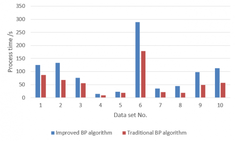
The process time of our algorithm is compared with that of the traditional BP algorithm in Figure 5. It can be seen that, in the same hardware environment, our algorithm consumed slightly more time than the traditional BP algorithm. However, a slightly longer process time is nothing compared with the obvious superiority in accuracy.
Table 2. Comparison of the accuracy of the two algorithms
|
Dataset number |
Accuracy of common BP algorithm |
Accuracy of proposed algorithm |
|
Dataset 1 |
99.38% |
99.41% |
|
Dataset 2 |
93.65% |
97.25% |
|
Dataset 3 |
96.62% |
97.18% |
|
Dataset 4 |
100% |
100% |
|
Dataset 5 |
97.53% |
97.61% |
|
Dataset 6 |
89.32% |
90.05% |
|
Dataset 7 |
98.61% |
98.72% |
|
Dataset 8 |
66.90% |
72.28% |
|
Dataset 9 |
77.59% |
82.30% |
|
Dataset 10 |
92.71% |
93.88% |
Figure 5. Comparison of process time of the two algorithms
Inspired by the theory of batch learning BP algorithm, this paper combines the LMS algorithm and the traditional BP algorithm into an improved classification algorithm for the MLP. The improved algorithm fully integrates the batch learning rules and momentum factor. To verify its effectiveness, the improved BP algorithm was compared with the traditional BP algorithm through experiments. The comparison shows that our algorithm clearly outperformed the traditional BP algorithm in classification accuracy. The research results shed new light on big data classification.
We want to thanks The Excellent Science and Technology Innovation Team of Jiangsu Universities and Colleges, the Application of Industrial Networks and Big Data; The Engineering Technology Research and Development Center of Jiangsu Higher Vocational and Technology Colleges, The Industrial Big Data and Intelligent Engineering Technology Research and Development Center; The Provincial Engineering Research Center of Jiangsu, the Innovation and Application of Jiangsu Small Business Industrial Internet Engineering Research Center.
The work is supported by "General program of natural science research in Jiangsu University, Research on Key Technologies of disaster tolerant mobile data collection for underwater acoustic sensor network, No. 19KJB520023"; "Open Lab of Edge of Computing for Smart Manufacturing, Changzhou College of Information Technology, Changzhou, China, KYPT201802Z".
[1] Yan, X., Jia, M. (2018). A novel optimized SVM classification algorithm with multi-domain feature and its application to fault diagnosis of rolling bearing. Neurocomputing, 313(3): 47-64. https://doi.org/10.1016/j.neucom.2018.05.002
[2] Zheng, B., Huang, H.Z., Guo, W., Li, Y.F., Mi, J. (2018). Fault diagnosis method based on supervised particle swarm optimization classification algorithm. Intelligent Data Analysis, 22(1): 191-210. https://doi.org/10.3233/IDA-163392
[3] Li, H.Y., Li, H.F., Wei, K.B. (2018). Automatic fast double KNN classification algorithm based on ACC and hierarchical clustering for big data. International Journal of Communication Systems, 31(16): e3488.1-e3488.11. https://doi.org/10.1002/dac.3488
[4] Brankovic, A., Falsone, A., Prandini, M., Piroddi, L. (2017). A feature selection and classification algorithm based on randomized extraction of model populations. IEEE Transactions on Cybernetics, 48(4): 1151-1162. https://doi.org/10.1109/TCYB.2017.2682418
[5] Kumar, M.A., Gopal, M. (2010). Fast multiclass SVM classification using decision tree based one-against-all method. Neural Processing Letters, 32(3): 311-323. https://doi.org/10.1007/s11063-010-9160-y
[6] Bazan, J.G., Bazan-Socha, S., Buregwa-Czuma, S., Dydo, L., Rzasa, W., Skowron, A. (2016). A classifier based on a decision tree with verifying cuts. Fundamenta Informaticae, 143(1-2): 1-18. https://doi.org/10.3233/FI-2016-1300
[7] Chandanapalli, S.B., Sreenivasa Reddy, E., Rajya Lakshmi, D. (2017). FTDT: Rough set integrated functional tangent decision tree for finding the status of aqua pond in aquaculture. Journal of Intelligent & Fuzzy Systems, 32(3): 1821-1832. https://doi.org/10.3233/JIFS-152634
[8] Hajisalem, V., Babaie, S. (2018). A hybrid intrusion detection system based on ABC-AFS algorithm for misuse and anomaly detection. Computer Networks, 136(5): 37-50. https://doi.org/10.1016/j.comnet.2018.02.028
[9] Bin, S., Sun, G.X., Cao, N., Qiu, J.M., Zheng, Z.Y., Yang, G.H., Zhao, H.Y., Jiang, M., Xu, L. (2019). Collaborative filtering recommendation algorithm based on multi-relationship social network. CMC-Computers, Materials & Continua, 60(2): 659-674. https://doi.org/10.32604/cmc.2019.05858
[10] Liang, T., Xu, X., Xiao, P. (2017). A new image classification method based on modified condensed nearest neighbor and convolutional neural networks. Pattern Recognition Letters, 94(7): 105-111. https://doi.org/10.1016/j.patrec.2017.05.019
[11] Ezghari, S., Zahi, A., Zenkouar, K. (2017). A new nearest neighbor classification method based on fuzzy set theory and aggregation operators. Expert Systems with Application, 80(9): 58-74. https://doi.org/10.1016/j.eswa.2017.03.019
[12] Yan, X., Jia, M. (2018). A novel optimized SVM classification algorithm with multi-domain feature and its application to fault diagnosis of rolling bearing. Neurocomputing, 313(11): 47-64. https://doi.org/10.1016/j.neucom.2018.05.002
[13] Sun, G.X., Bin, S. (2018). A new opinion leaders detecting algorithm in multi-relationship online social networks. Multimedia Tools and Applications, 77(4): 4295-4307. https://doi.org/10.1007/s11042-017-4766-y
[14] Rashed, M., Rashed, E.A. (2017). Double-Sided Sliding-Paraboloid (DSSP): A new tool for preprocessing GPR data. Computers & Geoences, 102(5): 12-21. https://doi.org/10.1016/j.cageo.2017.02.005
[15] Ramírez-Gallego, S., García, S., Benítez, J.M., Herrera, F. (2015). Multivariate discretization based on evolutionary cut points selection for classification. IEEE Transactions on Cybernetics, 46(3): 595-608. https://doi.org/10.1109/TCYB.2015.2410143
[16] Barbu, A.L., Laurent-Varin, J., Perosanz, F., Mercier, F., Marty, J.C. (2018). Efficient QR sequential least square algorithm for high frequency GNSS precise point positioning seismic application. Advances in Space Research, 61(1): 448-456. https://doi.org/10.1016/j.asr.2017.10.032
[17] Ding, S.F., Xu, L., Su, C.Y., Jin, F.X. (2012). An optimizing method of RBF neural network based on genetic algorithm. Neural Computing and Applications, 21(2): 333-336. https://doi.org/10.1007/s00521-011-0702-7