Approximate Solution of Linear Fredholm Integral Equation of the Second Kind Using Modified Simpson's Rule

Fredholm integral equations are a class of mathematical equations that arise in various branches of applied mathematics and engineering. These equations play a significant role in the study of boundary value problems, signal processing, quantum mechanics, and many other areas [1-3]. So approximate solution of linear Fredholm integral equation of the second kind is one of the most important subjects discussed in recent years, using different kind of methods such as Method of Moments, Variational Iteration Method [4].

Various methods, including iterative procedures, eigenfunction expansions, and numerical quadrature, are employed to find solutions to these equations. Many authors have extensively explored the approximate solutions of linear Fredholm integral equations of the second kind, utilizing a variety of quadrature methods. Such that Haar wavelets [5], hybrid functions [6], sinc-Galerkin method [7], sinc-collocation method [8], collocation methods based on cubic spline quadrature [9], collocation methods based on B-cubic spline quadrature [10], repeated modified trapezoid quadrature method [11, 12], Numerical solution of the Fredholm integral equations with a quadrature method [13], Bernoulli wavelet based numerical method for solving Fredholm integral equations of the second kind [14]. Malmir [15] used the numerical solution method based on Chebyshev and Legendre polynomials to solve the Fredholm integral equation of the second kind.

Each of these approaches offers unique advantages and has contributed to our understanding and practical implementation of approximate solutions for such integral equations.

In this study, we introduce a novel approach to obtain an approximate numerical solution of linear Fredholm integral equation of the second kind, which is given by the equation:

$\phi(x)-\int_a^b k(x, t) \phi(t) d t=f(x), a \leq x \leq b$              (1)

where, the function f(x) and the kernel k(x, t) are known, but ϕ(x) the exact solution is unknown and to be determined. We assume that the integral equation (1) has a unique solution. To find this solution numerically, we employ a modified numerical technique based on the quadrature Simpson's rule, this method is first proposed by Nadir and Rahmoune [16], for solving Volterra integral equations. The idea is to approximate the solution of the linear Fredholm integral equations in even number of equally spaced points. This technique will enable us to approximate the solution ϕ(x) efficiently and accurately.

The paper is organized into six sections. The second section presents the existence and uniqueness of a solution. In the third section, we delve into the algorithm used in our research method, providing a detailed explanation of its workings. A study of convergence is conducted in the fourth section. Section 5 is devoted to presenting a series of diverse examples that serve as practical tests for evaluating the method's performance and applicability. Finally, in the last section, conclusion of the proposed method is discussed.

Consider the linear Fredholm integral equation of the second kind with regular kernels (non- singular):

$\phi(x)-\int_a^b k(x, t) \phi(t) d t=f(x), a \leq x \leq b$                 (2)

where, $a, b \in \mathbb{R}$, f(x) is a known continuous function on the finite interval [a, b], the kernel k(x, t) is known and continuous function in [a, b]×[a, b] but ϕ(x) the exact solution of the equation (1) is an unknown continuous function in [a, b] to be determined.

Let $a=x_0<x_1<\ldots<x_{2 i-1}<x_{2 i}<\ldots<x_{2 n}=b$, be a subdivision of the interval [a, b], with $h=\frac{b-a}{2 n}$.  

We approximate the right-hand integral (1) at the even point (x_2i) with the Simpson's quadrature rule, we have:

$\phi\left(x_{2 i}\right)-\int_a^b k\left(x_{2 i}, t\right) \phi(t) d t=f\left(x_{2 i}\right)$,

$\phi\left(x_{2 i}\right)-\sum_{j=0}^{j=n-1} \int_{x_{2 j}}^{x_{2 j+2}} k\left(x_{2 i}, t\right) \phi(t) d t=f\left(x_{2 i}\right)$,

i=0, 1, ..., n

$\begin{gathered}\phi_{2 i}-\frac{h}{3} \sum_{j=0}^{j=n-1}\left(k_{2 i, 2 j} \phi_{2 j}+4 k_{2 i, 2 j+1} \phi_{2 j+1}+\right.  \left.k_{2 i, 2 j+2} \phi_{2 j+2}\right)=f_{2 i}\end{gathered}$

For a smaller step h, an approximation to ϕ_2i can be computed by replacing ϕ_2j+1 by the average $\frac{\phi_{2 j}+\phi_{2 j+2}}{2}$.

$\begin{array}{r}\phi_{2 i}-\frac{h}{3} \sum_{j=0}^{j=n-1}\left(k_{2 i, 2 j} \phi_{2 j}+4 k_{2 i, 2 j+1} \frac{\phi_{2 j}+\phi_{2 j+2}}{2}+k_{2 i, 2 j+2} \phi_{2 j+2}\right)=f_{2 i}\end{array}$

or

$\begin{gathered}\phi_{2 i}-\frac{h}{3} \sum_{j=0}^{j=n-1}\left[\left(k_{2 i, 2 j}+2 k_{2 i, 2 j+1}\right) \phi_{2 j}+\left(k_{2 i, 2 j+2}+\right.\right.\left.\left.2 k_{2 i, 2 j+1}\right) \phi_{2 j+2}\right]=f_{2 i}\end{gathered}$

then

$\begin{gathered}\phi_{2 i}-\frac{h}{3} \sum_{j=0}^{j=n-1}\left(k_{2 i, 2 j}+2 k_{2 i, 2 j+1}\right) \phi_{2 j}-\frac{h}{3} \sum_{j=0}^{j=n-1}\left(k_{2 i, 2 j+2}+\right. \left.2 k_{2 i, 2 j+1}\right) \phi_{2 j+2}=f_{2 i}\end{gathered}$

$\begin{gathered}\phi_{2 i}-\frac{h}{3} \sum_{j=0}^{j=n-1}\left(k_{2 i, 2 j}+2 k_{2 i, 2 j+1}\right) \phi_{2 j}-\frac{h}{3} \sum_{j=1}^{j=n}\left(k_{2 i, 2 j}+\right.  \left.2 k_{2 i, 2 j-1}\right) \phi_{2 j}=f_{2 i}\end{gathered}$

for i=0, ..., n, we get the following system:

$\begin{gathered}\phi_{2 i}-\frac{h}{3}\left(k_{2 i, 0}+2 k_{2 i, 1}\right) \phi_0-\frac{2 h}{3} \sum_{j=1}^{j=n-1}\left(k_{2 i, 2 j-1}+k_{2 i, 2 j}+\right.\left.k_{2 i, 2 j+1}\right) \phi_{2 j}-\frac{h}{3}\left(2 k_{2 i, 2 n-1}+k_{2 i, 2 n}\right) \phi_{2 n}=f_{2 i}\end{gathered}$ 

With 2n+1 equation, and 2n+1 unknowns.

The objective of this section is to demonstrate the efficacy of the method outlined in the paper through a series of numerical experiments.

Example 1.

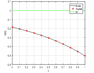
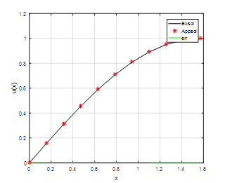
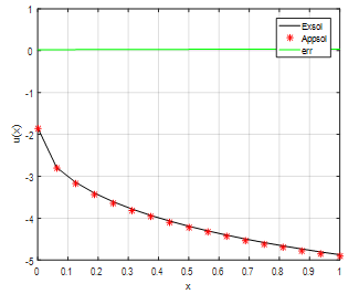
Let us consider the Fredholm integral equation of the second kind $\phi(x)-\int_0^1 2 \exp (x+t) \phi(t) d t=\exp (x), 0 \leq x \leq 1$ the exact solution ϕ_ex(x) is given by $\phi_{e x}(x)=\frac{\exp (x)}{2-\exp (2)}$.

Table 1 and Figure 1 present the exact, approximate solutions and the absolute error |ϕ_app-ϕ_ex(x)| for n=10 of the equation in the Example 1 obtained by the modified Simpson's rule, in some arbitrary points.

Table 1. Numerical results for n=10 in example 1

tu_pian_1.png

Figure 1. Exact, approximate solutions and absolute error (n=10) for example 1

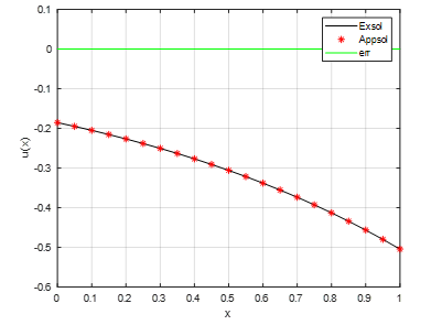
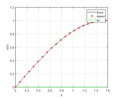
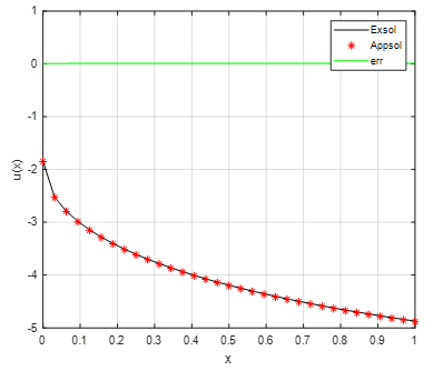
Table 2 and Figure 2 present the exact, approximate solutions and the absolute error |ϕ_app-ϕ_ex(x)| for n=20 of the equation in the Example 1 obtained by the modified Simpson’s rule, in some arbitrary points.

Table 2. Numerical results for n=20 in example 1

tu_pian_2.png

Figure 2. Exact, approximate solutions and absolute error (n=20) for example 1

Example 2.

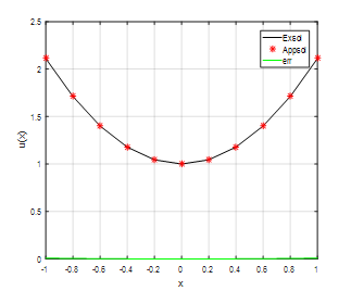
Consider the linear Fredholm integral equation of the second kind $\phi(x)-\int_{-1}^1\left(x t+x^2 t^2\right) \phi(t) d t=1,-1 \leq x \leq 1$. The exact solution ϕ_ex(x) is given by $\phi_{e x}(x)=1+\frac{10}{9} x^2$.

Table 3 and Figure 3 present the exact, approximate solutions and the absolute error |ϕ_app-ϕ_ex(x)| for n=10 of the equation in the Example 2 obtained by the modified Simpson's rule, in some arbitrary points.

Table 3. Numerical results for n=10 in example 2

tu_pian_3.png

Figure 3. Exact, approximate solutions and absolute error (n=10) for example 2

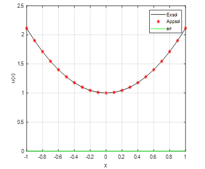
Table 4 and Figure 4 present the exact, approximate solutions and the absolute error |ϕ_app-ϕ_ex(x)| for n=20 of the equation in the Example 2 obtained by the modified Simpson's rule, in some arbitrary points.

Table 4. Numerical results for n=20 in example 2

tu_pian_4.png

Figure 4. Exact, approximate solutions and absolute error (n=20) for example 2

Example 3.

Consider the linear Fredholm integral equation of the second kind $\phi(x)-\int_0^{\frac{\pi}{2}} \frac{4}{\pi} \cos (x-t) \phi(t) d t=-\frac{2}{\pi} \cos (x)$, $0 \leq x \leq \frac{\pi}{2}$ the exact solution ϕ_ex(x) is given by ϕ_ex(x)=sin(x).

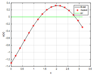
Table 5 and Figure 5 present the exact, approximate solutions and the absolute error |ϕ_app-ϕ_ex(x)| for n=10 of the equation in the Example 3 obtained by the modified Simpson's rule, in some arbitrary points.

Table 5. Numerical results for n=10 in example 3

tu_pian_5.png

Figure 5. Exact, approximate solutions and absolute error (n=10) for example 3

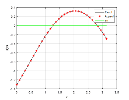
Table 6 and Figure 6 present the exact, approximate solutions and the absolute error |ϕ_app-ϕ_ex(x)| for n=20 of the equation in the Example 3 obtained by the modified Simpson's rule, in some arbitrary points.

Table 6. Numerical results for n=20 in example 3

tu_pian_6.png

Figure 6. Exact, approximate solutions and absolute error (n=20) for example 3

In the following examples, a comparison with the least-squares and polynomial method [19] is done.

Example 4.

Consider the linear Fredholm integral equation of the second kind [19] $\phi(x)-\int_0^1(\sqrt{x}+\sqrt{t}) \phi(t) d t=1+x, 0 \leq x \leq 1$, the exact solution ϕ_ex(x) is given by $\phi_{e x}(x)=\frac{-129}{70}-\frac{141}{35} \sqrt{x}+x$.

Numerical results for n=16 of the equation in the Example 4 obtained by the modified Simpson's method, in some arbitrary points are presented in Table 7 and Figure 7, a comparison of obtained results with ones obtained by least-squares [19], is given in Table 7.

Table 7. Comparison of results for n=16 in example 4

tu_pian_7.png

Figure 7. Exact, approximate solutions and absolute error (n=16) for example 4

Numerical results for n=32 of the equation in the Example 4 obtained by the modified Simpson's method, in some arbitrary points are presented in Table 8 and Figure 8, a comparison of obtained results with ones obtained by polynomial method |ϕ-ϕ₂| [19], is given in Table 8.

Table 8. Comparison of results for n=32 in example 4

tu_pian_8.png

Figure 8. Exact, approximate solutions and absolute error (n=32) for example 4

Example 5.

In the final example, we apply our approach to the integral equation [19] $\phi(x)-\int_0^\pi(\cos (x)+\cos (t)) \phi(t) d t=\sin (x), 0 \leq x \leq \pi$ to approximate the unique solution $\phi_{e x}(x)=\sin (x)+\frac{4}{2-\pi^2} \cos (x)+\frac{2 \pi}{2-\pi^2}$.

Numerical results for n=16 of the equation in the Example 5 obtained by the modified Simpson's method, in some arbitrary points are presented in Table 9 and Figure 9, a comparison of obtained results with ones obtained by least-squares [19], is given in Table 9.

Table 9. Comparison of results for n=16 in example 5

tu_pian_9.png

Figure 9. Exact, approximate solutions and absolute error (n=16) for example 5

Numerical results for n=32 of the equation in the Example 5 obtained by the modified Simpson's method, in some arbitrary points are presented in Table 10 and Figure 10, a comparison of obtained results with ones obtained by polynomial method |ϕ-ϕ₂| [19], is given in Table 10.

Table 10. Comparison of results for n=32 in example 5

tu_pian_10.png

Figure 10. Exact, approximate solutions and absolute error (n=32) for example 5