Fikri Badru Salam![]() | Dina Tri Utari*
| Dina Tri Utari*![]()
© 2024 The authors. This article is published by IIETA and is licensed under the CC BY 4.0 license (http://creativecommons.org/licenses/by/4.0/).
OPEN ACCESS
Schizophrenia is a severe mental illness, the main symptoms of which include delusions, hallucinations, and cognitive disturbances. This disease can affect the quality of human life. Schizophrenia affects around 24 million people worldwide. This study involved 14 patients with paranoid schizophrenia and 14 healthy controls with 19 channels. This study aims to apply the Long Short-Term Memory (LSTM) method to Electroencephalography (EEG) signals for classifying people with schizophrenia. EEG signal analysis uses a bandpass filter with an interval frequency of 0.5 – 45 Hz with a maximum EEG segment duration of 5 seconds with an overlap of 1 second. Feature extraction used is based on Frequency-Domain Features. The data is standardized with a scaler by dividing training, validation, and testing data by 80%, 15%, and 15%, with a random state 42. The dense layer uses one layer LSTM, Dropout of 0.25, and Activation ReLu and Adam optimization. Therefore, the model accuracy is 99.94%. The K-Fold Cross Validation evaluation matrix results for the validation dataset are 98.18%. From the selected model, predictions were made using data testing to obtain an evaluation matrix for the diagnosis of schizophrenia, including a precision of 95%, recall of 93%, F1-score of 94%, and accuracy of 94%. Hence, in this study, it is evident that LSTM demonstrates effectiveness in accurately classifying schizophrenia patients using their brainwave data.
schizophrenia, electroencephalography, band pass filtering, neural network, Long Short-Term Memory
Schizophrenia is a complex mental disorder characterized by abnormal thoughts, perceptions, and behaviors. An early and accurate diagnosis of schizophrenia is crucial for effective treatment and management. Electroencephalography (EEG) signals provide valuable insights into the brain activity of individuals, offering a potential avenue for understanding and classifying schizophrenia.
An EEG is a device that examines images of recorded electrical activity in the brain, explaining its functionality and interpretation [1]. The recording of EEG signals affixed to the scalp provides information about brain wave patterns associated with various mental states and psychiatric disorders. This non-invasive technique is performed by placing conductive electrodes on the scalp, usually using an electrode cap for multichannel recording. These electrodes read the brain’s electrical signals from the surface of the head, which are amplified from microvolt magnitudes to a range in which they can be digitized and accurately stored [2].
The motivation behind utilizing Long Short-Term Memory (LSTM) for schizophrenia patient classification through EEG signal analysis lies in LSTM networks’ ability to capture temporal dependencies and patterns in sequential data. EEG signals are time-varying and exhibit complex temporal dynamics, making LSTM suitable for modeling and analyzing these signals. Previous research has demonstrated the potential of LSTM and related deep learning techniques in various mental health applications and EEG analysis applications. For instance, Liu et al. introduced a classification technique for schizophrenia using individual hierarchical brain networks derived from structural MRI images. They demonstrated the effectiveness of incorporating hierarchical network structures and correlations between regions of interest in improving classification accuracy [3].
Furthermore, Prabhakar et al. explored the classification of schizophrenia EEG signals using swarm intelligence computing and optimization algorithms. They achieved promising results in accurately distinguishing between typical and schizophrenia cases, highlighting the potential of advanced computational techniques in EEG-based classification [4]. In addition, brain activity and EEG signal analysis have been widely used in studying various mental disorders, including stress [5]. The classification of stress using brain signals based on LSTM networks demonstrates the potential of LSTM in capturing and analyzing complex brain patterns associated with mental health conditions [5].
In this study, we used LSTM to analyze EEG signals to classify patients effectively. The LSTM model excels in interpreting the processed EEG signal data, facilitating accurate patient classification. This research incorporates feature extraction techniques and bandpass filtering to improve EEG signal quality and ensure reliability. This approach carefully filters out noise, ensuring that the EEG waveforms used in the LSTM analysis have the highest precision and accuracy.
By leveraging the capabilities of LSTM networks, this research aims to contribute to developing a reliable and accurate classification model for schizophrenia using EEG signals. Analyzing EEG signals with LSTM can provide insights into the temporal dynamics and patterns associated with schizophrenia, enabling improved diagnosis and understanding of the disorder.
This study mainly used basic frequency domain features for feature extraction from EEG signals. However, it is worth considering the application of more advanced feature extraction techniques, such as wavelet transform and Fast Fourier Transform (FFT), which may offer deeper insights or better performance.
In addition, the segmentation process of the EEG signal plays a vital role in the model’s effectiveness. In particular, decisions about the degree of overlap and the duration of the signal segments significantly impact the model’s accuracy. Higher overlap values in signal segments improve model performance, allowing for more comprehensive data utilization. Conversely, shorter signal segment lengths are generally more effective, as they provide better resolution and capture more detailed features of the EEG signal. These segmentation parameters must be carefully optimized to balance the trade-offs and achieve the best model performance.
This study uses a dataset provided in 2017, which the public can access on the RepOD website. There are two categories: patients with paranoid schizophrenia and healthy patients as a control group. The study sample consisted of 14 patients with paranoid schizophrenia (seven men and seven women aged 24-32) from the Institute of Psychiatry and Neurology in Warsaw, Poland, and 14 healthy controls (seven men aged 23-30 and seven women aged 25-32).
The patients meet the criteria for paranoid schizophrenia (ICD-10 category F20.0). The Institute of Psychiatry and Neurology Ethics Committee approved the study plan in Warsaw. All participants received a written explanation of the protocol and gave written informed consent to participate in the study. The inclusion criteria were a minimum age of 18 years, a diagnosis of F20.0 according to ICD-10, and a seven-day withdrawal period. Exclusion criteria included pregnancy, organic brain pathology, severe neurological diseases (such as epilepsy, Alzheimer’s, or Parkinson’s), general medical disorders, and early-stage schizophrenia (first episode of schizophrenia). Fourteen patients who finished the study were paired based on gender and age in the control group [6].
The dataset accessed from this website consists of files in the European Data Format (EDF), a widely recognized standard for storing and exchanging medical time series data. Each file in this collection is carefully labeled to distinguish between control subjects and schizophrenia patients, thus facilitating clear and organized analysis.
However, it is essential to note that this website lacks specific information regarding the demographic matching of the two groups, especially regarding gender and age. This absence of detailed demographic matching may affect the findings of the study. In addition, this website adheres to strict privacy protection protocols, ensuring that all patient data remains confidential and secure under privacy standards. This aspect underscores the ethical consideration given to patient information while still providing valuable data for research purposes.
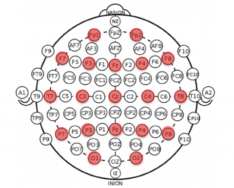
Each subject had their eyes closed at rest while fifteen minutes of EEG data were recorded. The data was collected at a sampling rate of 250 Hz utilizing a conventional 10-20 EEG configuration with 19 EEG channels: Fp1, Fp2, F7, F3, Fz, F4, F8, T3, C3, Cz, C4, T4, T5, P3, Pz, P4, T6, O1, O2. The reference electrode is positioned at FCz, as depicted in Figure 1.
Figure 1. EEG channel [7]
EEG data analysis involves artifact-free segments lasting over thirty seconds, excluding eye movements, cardiac activity, and muscle contractions. Each EEG channel’s signal was filtered using a second-order Butterworth filter within a specific physiological frequency range. The frequency ranges are as follows: The frequency ranges for different brain waves are as follows: delta waves 2-4 Hz, theta waves 4.5-7.5 Hz, alpha waves 8-12.5 Hz, beta waves 13-30 Hz, and gamma waves 30-45 Hz [8].
3.1 EEG segmentation process
The fluctuation of statistical properties of the EEG signal over time intervals causes it to be non-stationary [9]. The solution to this difficulty is to break long EEG signal sequences into short-duration segments considered pseudo-stationary with identical statistical temporal and frequency properties [10]. This study utilizes a method that segments the EEG data from different psychotic intervals into shorter duration segments ranging from 5 to 50 seconds with no overlap.
Although the CHB-MIT dataset contains EEG signals with lengths ranging from a few minutes to several hours, this study only analyzes a maximum EEG segment duration of 5 seconds. This is because increasing segment duration further results in a small number of EEG samples, which needs to be improved for adequate training, testing, and validation of the suggested categorization. In addition, this shorter time segment benefits from reduced computational power, transmission bandwidth, and storage requirements [11].
3.2 Feature extraction
The most significant aspect of the study, particularly in EEG signals analysis, is feature extraction. This is because feature selection determines how the data distribution pattern is described, and this model influences the classification technique utilized. Feature extraction primarily aims to reduce complex EEG data to a more compact representation while maintaining crucial information for subsequent analysis or categorization. Different feature extraction techniques are utilized depending on needs, including time-domain features, frequency-domain features, time-frequency features, and nonlinear features.
Statistical measures such as mean, median, variance, standard deviation, skewness, and kurtosis are components of the frequency-domain [12].
(1) Mean
The mean is the average value of each data channel for each participant. This study computes the mean to symbolize the value of each channel.
$\bar{x}=\frac{\sum_{i=1}^n x_i}{n}$ (1)
(2) Variance
The measurement of variance shows how far the spread of a set of data of each channel is.
$\sigma^2=\frac{\sum_{i=1}^n\left(x_i-\bar{x}\right)^2}{n-1}$ (2)
(3) Standard deviation
The standard deviation (STD) quantifies the amount of dispersion or variation in each channel from its mean.
$S T D=\sqrt{\frac{\sum_{i=1}^n\left(x_i-\bar{x}\right)^2}{n-1}}$ (3)
(4) Minimum
Each channel can be analyzed to determine the minimum or value.
(5) Maximum
The maximum value for each channel is the most significant value that can be represented in that channel.
(6) Kurtosis
Kurtosis is the statistical measure that describes the peakedness or flatness of a distribution of values in each channel [13].
$K=\frac{\frac{1}{n} \sum_{i=1}^n\left(x_i-\bar{x}\right)^4}{\left(\frac{1}{n} \sum_{i=1}^N\left(x_i-\bar{x}\right)^2\right)^2}-3$ (4)
(7) Skewness
Skewness is a metric that indicates the degree of similarity or asymmetry in each channel’s distribution [13].
$K=\frac{\frac{1}{n} \sum_{i=1}^N\left(x_i-\bar{x}\right)^3}{\left(\frac{1}{n-1} \sum_{i=1}^N\left(x_i-\bar{x}\right)^2\right)^{2 / 3}}-3$ (5)
(8) Root Mean Square (RMS)
RMS is a standard EEG signal analysis method. RMS is a mathematical calculation that measures the amplitude or overall power of a time series signal, in this case, an EEG signal. The RMS value measures the overall energy or amplitude of the EEG signal. This can be useful in various EEG applications, such as identifying specific patterns of brain activity, detecting anomalies, or monitoring changes in brain activity over time.
$R M S=\sqrt{\frac{\sum_{i=1}^n x_i^2}{n}}$ (6)
3.3 Long-Short Term Memory (LSTM)
LSTM is a Recurrent Neural Network (RNN) capable of capturing long-term dependencies within data sequences by retaining information for an extended duration, thus mitigating the issue of vanishing gradients commonly found in RNNs [14]. Hochreiter and Schmidhuber pioneered the LSTM network [15]. This network is commonly used to classify time sequence data, speech data, audio, text, and biological signals, among other things [16, 17].
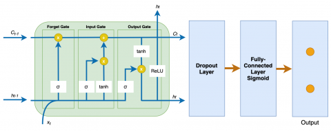
Figure 2. LSTM basic architecture [11]
According to Figure 2, the LSTM architecture is characterized by a primary LSTM cell composed of three gates that control the flow of information from one cell state to the next. There are forget, input, and output gates [15, 18]. The three gates employ sigmoid activation to regulate the information flow. The forget gate determines whether the information in each data sample should be kept or discarded. The gate considers the current input signal xt and the previous output sequence yt-1 in cell Ct-1 to generate an output ft ranging from 0 to 1, whereas 0 signifies a complete information forget gate, while 1 indicates a complete information storage gate.
The input gate determines whether to retain information in the current cell Ct by multiplying its output with the tanh activation layer $\tilde{C}_t$. The output gate regulates the flow of specific information yt in Ct at the LSTM cell’s output by merging its output Ot with another tanh activation layer. The action of the three LSTM cell gates creates the output yt in cell Ct , which is stated mathematically by the following equations [18]:
$\sigma(x)=\frac{1}{1+e^{-x}}$ (7)
$\tanh (x)=2 \sigma(2 x)-1$ (8)
$f_t=\sigma\left(W_f \cdot\left[h_{t-1}, x_t\right]+b_f\right)$ (9)
$i_t=\sigma\left(W_i \cdot\left[h_{t-1}, x_t\right]+b_i\right)$ (10)
$\tilde{C}_t=\tanh \left(W_f\left[h_{t-1}, x_t\right]+b_C\right)$ (11)
$C_t=f_t * C_{t-1}+i_t * \tilde{C}_t$ (12)
$o_t=\sigma\left(W_o \cdot\left[h_{t-1}, x_t\right]+b_o\right)$ (13)
$h_t=o_t * \tanh C_t$ (14)
${ReLU}=\max (0, x)=\left\{\begin{array}{c}\alpha x \text { if } x \leq 0 \\ x \text { if } x \geq 0\end{array}\right.$ (15)
where, σ is the sigmoid function, ft is the forget gate, it is the input gate, ot is the output gate, W and b are the weight matrix and bias factor for different gates in the LSTM cell. Moreover, ht-1 is the output value before the t order, Ct-1 is the cell state before the t order (initial value for ht-1=0 and Ct-1=0 [19]), the value of tanh(x) between the interval -1 to 1, α is 0 for ReLU [20].
4.1 Data overview
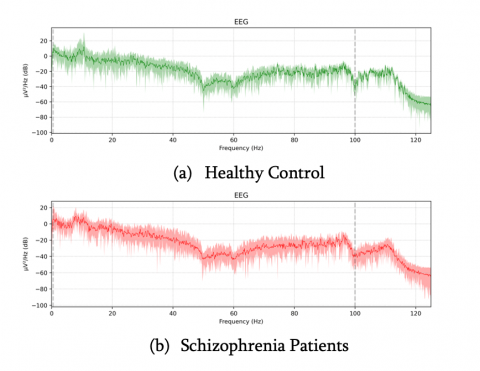
Fourteen patients with paranoid schizophrenia were compared to 14 healthy individuals in this study. Data was gathered at a sampling frequency of 250 Hz utilizing a traditional 10-20 EEG setup with 19 channels. Figure 3. illustrates the EEG signals of healthy individuals and patients with schizophrenia.
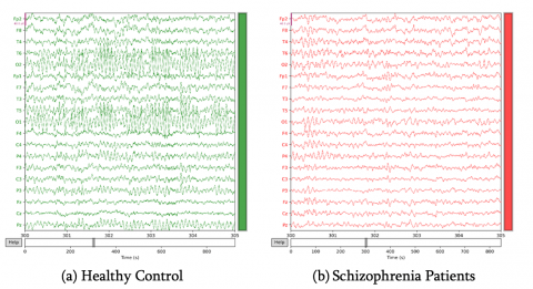
Figure 3 shows that the data of healthy controls and schizophrenia patients at each frequency shows a difference where the decrease in the value of Power Spectral Density (PSD) drastically decreases at specific frequencies such as when the frequency is from 100 Hz to 120 Hz. Then as an example of the waves for each channel it is shown in Figure 4. From Figure 4, there are abnormalities in schizophrenia patients. In the EEG wave signals of schizophrenia patients, brain activity tends to show regular and coordinated patterns. Whereas in the EEG signal waves of healthy control patients, brain activity patterns often show significant changes due to electrical activity in the brain. This shows that the activity of the structure and function of the brain in patients with schizophrenia is not regular.
Figure 3. EEG signal data for healthy and schizophrenia patients
Figure 4. EEG signal data at 300–305 second
4.2 Bandpass filtering, EEG segmentation, and feature extraction
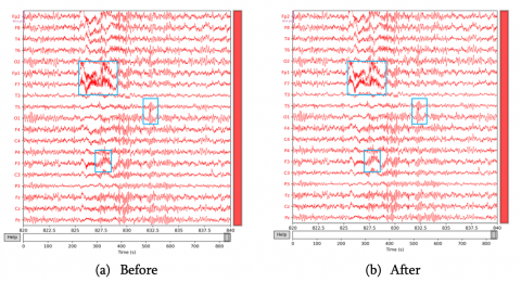
The EEG signal data collected by the instrument from schizophrenia patients and healthy controls must be free of artifacts and noise before being processed for schizophrenia prediction, necessitating precise filters. We apply a Butterworth bandpass filter to multichannel EEG signals with a frequency range of 0 Hz to 45 Hz. This method is preferred in biomedical signal analysis because of its flat and wave-free frequency response. Figure 5 shows an example of EEG signal data processed using bandpass filtering.
Figure 5. EEG data before and after bandpass filter
In Figure 5, the EEG signal with a bandpass filter of 0.5–45 Hz shows a difference in the resulting wave pattern. The waveforms are generated at diverse frequencies in the EEG signal before the bandpass filter is performed. In contrast, when the bandpass filter is applied, the signal wave is more tenuous, where the frequencies outside 0.5–45 Hz are removed. Then after the bandpass filter is carried out, it will enter the epoching or EEG segmentation process.
Since the statistical properties of the EEG signal vary, it is non-stationary [9]. Extended EEG signals are segmented into brief sections assumed to be pseudo-stationary, displaying comparable statistical temporal and frequency characteristics [10]. This study also uses this method, which divides the EEG signals from distinct schizophrenic intervals into shorter segments. This study solely considers the maximal EEG segment duration of 5 seconds with a 1 second overlap. This is because increasing the segment time further results in a limited sample of the EEG data, which needs to be improved for adequate training, testing, and validation of the suggested categorization. Moreover, this shorter segment benefits from decreased processing computational power needs, reduced transmission bandwidth needs, and lower storage demands on local or cloud-based storage. The signal length is 1,250 points and total sample is 7,201 based on the bandpass filter and EEG segmentation results.
Eight statistical features were extracted for each channel, meaning 19 channels for each experiment; 152 features were extracted for each experiment in the EEG signal.
4.3 Classification using LSTM
When classifying EEG signals with the LSTM, the data is standardized on a scaler by splitting training and testing data by 80% training, 15% validation, and 15% testing with random state 42. The sequential LSTM model is utilized. In the sequential model, each layer is created individually, one after the other. The model sequentially processes data from input to output via a predetermined sequence of layers.
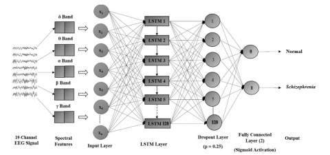
In the case of LSTM, we added an LSTM layer and other layers such as Dense of 1 (which employs one layer of LSTM), Dropout of 0.25, and Activation ReLu to the model. The LSTM model is optimized using binary cross entropy as the loss function. Adam’s optimizer integrates momentum method and adaptive learning rate and it adjusts the weights and biases of the model according to the gradient of the loss function. With a batch size of 32, the LSTM model was trained for 50 epochs. Figure 6 depicts the LSTM architectural model.
The LSTM model’s architecture in Figure 6 involves bandpass filtering 19 wave channels based on specific frequency ranges: 2–4 Hz (delta), 4.5–7.5 Hz (theta), 8–12.5 Hz (alpha), 13–30 Hz (beta), and 30–45 Hz (gamma). EEG segmentation is performed based on available data. The data input layer is 5,761 data, the LSTM layer is 128 units, the Dropout is 128, and the classification results are 0 which means healthy control and 1, for schizophrenia patients. The results of the LTSM model are shown in Table 1.
Figure 6. LSTM architecture
Table 1. LSTM results
|
Layer (type) |
Output Shape |
Parameter |
|
LSTM |
(None, 128) |
143,872 |
|
Dense |
(None, 1) |
129 |
|
Dropout |
(None, 128) |
0 |
According to Table 1, the LSTM model was chosen with the output shape (None, 128) and a total model parameter of 143,872 in LSTM modeling, which includes weight and bias. Then dense is one layer used in neural networks to conduct mathematical operations such as multiplication matrices between inputs and weights and bias addition. A dense layer is fully or partially linked to all neurons in the previous and subsequent layers. The dense layer in this study has 1 unit neuron, a dropout of 0.25, and employs the sigmoid activation function to create an output between 0 and 1.
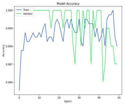
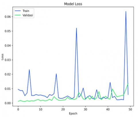
The model accuracy of the LSTM model utilized is 99.94%. The accuracy value for the validation dataset in the evaluation matrix using the K-Fold Cross Validation method with a K=5 is 98.18%. The accuracy and loss plots for each epoch up to epoch 50 are then examined, and the accuracy and loss results for the training and validation data LTSM model are obtained, as shown in Figure 7.
From Figure 7, there are several accuracy peaks, but the model we use is obtained by storing the model weights at the most significant peaks.
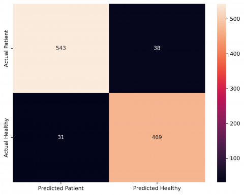
After we get the best model, we test the model for the predictive value of the testing data to get a confusion matrix which aims to be an evaluation tool used to measure the performance of a classification model.
From the confusion matrix, we perform a classification report to evaluate the method used to analyze and report the predicted results of a classification model. We get the precision of 95%, recall of 93%, F1-score of 94%, 581 support, and accuracy of 94% as shown in Figure 8.
Figure 7. Accuracy and loss plot on the LSTM model
Figure 8. Confusion matrix for testing data
The approach method employed in studying EEG signals to diagnose schizophrenia patients entails multiple steps. First, a bandpass filter in the 0.5–45 Hz frequency range filters out the delta, theta, alpha, beta, and gamma waves in the EEG data. The EEG signal is then segmented into shorter segments with a maximum duration of 5 seconds and an overlap of 1 second using the EEG segmentation procedure. Max, min, kurtosis, skewness, root mean square, mean, variance, and standard deviation are statistical features retrieved from EEG data. In each experiment, 152 characteristics were collected from 19 channels of EEG signals. This approach, which gets a classification accuracy of 94%, serves as the foundation for further EEG data analysis to identify schizophrenic patients.
[1] Winterer, G., McCarley, R.W. (2011). Electrophysiology of schizophrenia. In Schizophrenia. Wiley-Blackwell, Oxford, pp. 311-333.
[2] Teplan, M. (2002). Fundamentals of EEG measurement. Measurement Science Review, 2(2): 1-11.
[3] Liu, J., Li, M., Pan, Y., Wu, F.X., Chen, X., Wang, J. (2017). Classification of schizophrenia based on individual hierarchical brain networks constructed from structural MRI images. IEEE Transactions on NanoBioscience, 16(7): 600-608. https://doi.org/10.1109/TNB.2017.2751074
[4] Prabhakar, S.K., Rajaguru, H., Kim, S.H. (2020). Schizophrenia EEG signal classification based on swarm intelligence computing. Computational Intelligence and Neuroscience, 2020: 8853835. https://doi.org/10.1155/2020/8853835
[5] Phutela, N., Relan, D., Gabrani, G., Kumaraguru, P., Samuel, M. (2022). Stress classification using brain signals based on LSTM Network. Computational Intelligence and Neuroscience, 2022: 7607592. https://doi.org/10.1155/2022/7607592
[6] Olejarczyk, E., Jernajczyk, W. (2017). Graph-based analysis of brain connectivity in schizophrenia. PLoS One, 12(11): e0188629. https://doi.org/10.1371/journal.pone.0188629
[7] Kang, X., Agastya, I.M.A., Handayani, D.O.D., Kit, M.H., Rahman, A.W.B.A. (2021). Electroencephalogram (EEG) dataset with porn addiction and healthy teenagers under rest and executive function task. Data Brief, 39: 107467. https://doi.org/10.1016/j.dib.2021.107467
[8] Luján, M., Jimeno, M., Mateo Sotos, J., Ricarte, J., Borja, A. (2021). A survey on EEG signal processing techniques and machine learning: Applications to the neurofeedback of autobiographical memory deficits in schizophrenia. Electronics (Basel), 10(23): 3037. https://doi.org/10.3390/electronics10233037
[9] Singh, K., Singh, S., Malhotra, J. (2021). Spectral features based convolutional neural network for accurate and prompt identification of schizophrenic patients. Proceedings of the Institution of Mechanical Engineers, Part H: Journal of Engineering in Medicine, 235(2): 167-184. https://doi.org/10.1177/0954411920966937
[10] Barlow, J.S. (1985). Methods of analysis of nonstationary EEGs, with emphasis on segmentation techniques. Journal of Clinical Neurophysiology, 2(3): 267-304. https://doi.org/10.1097/00004691-198507000-00005
[11] Singh, K., Malhotra, J. (2022). Two-layer LSTM network-based prediction of epileptic seizures using EEG spectral features. Complex & Intelligent Systems, 8(3): 2405-2418. https://doi.org/10.1007/s40747-021-00627-z
[12] Stancin, I., Cifrek, M., Jovic, A. (2021). A review of eeg signal features and their application in driver drowsiness detection systems. Sensors, 21(11): 3786. https://doi.org/10.3390/s21113786
[13] Zhang, G., Davoodnia, V., Sepas-Moghaddam, A., Zhang, Y., Etemad, A. (2019). Classification of hand movements from EEG using a deep attention-based LSTM network. arXiv, 1-9. https://doi.org/10.1109/JSEN.2019.2956998
[14] Graves, A., Schmidhuber, J. (2005). Framewise phoneme classification with bidirectional LSTM and other neural network architectures. Neural Networks, 18(5-6): 602-610. https://doi.org/10.1016/j.neunet.2005.06.042
[15] Hochreiter, S., Schmidhuber, J. (1997). Long short-term memory. Neural Comput, 9(8): 1735-1780. https://doi.org/10.1162/neco.1997.9.8.1735
[16] Yildirim, Ö. (2018). A novel wavelet sequence based on deep bidirectional LSTM network model for ECG signal classification. Computers in Biology and Medicine, 96: 189-202. https://doi.org/10.1016/j.compbiomed.2018.03.016
[17] Connor, J.T., Martin, R.D., Atlas, L.E. (1994). Recurrent neural networks and robust time series prediction. IEEE Transactions on Neural Networks, 5(2): 240-254. https://doi.org/10.1109/72.279188
[18] Baratloo, A., Hosseini, M., Negida, A., El Ashal, G. (2015). Part 1: Simple definition and calculation of accuracy, sensitivity and specificity. [Online]. Available: https://www.jemerg.com.
[19] Lubis, N.H., Lubis, Y.F.A. (2021). Implementasi model recurrent neural network dalam melakukan prediksi harga kartu perdana internet dengan menggunakan algoritma long short term memory. In Prosiding SNASTIKOM: Seminar Nasional Teknologi Informasi & Komunikasi, pp. 463-469.
[20] Tilaver, H., Salti, M., Aydogdu, O., Kangal, E.E. (2021). Deep learning approach to Hubble parameter. Computer Physics Communications, 261: 107809. https://doi.org/10.1016/j.cpc.2020.107809