Saravanan Vadivel![]() | Poongothai Venugopal
| Poongothai Venugopal![]() | Godhandaraman Pakkirisamy*
| Godhandaraman Pakkirisamy*![]()
© 2024 The authors. This article is published by IIETA and is licensed under the CC BY 4.0 license (http://creativecommons.org/licenses/by/4.0/).
OPEN ACCESS
This article explores a M/M/m unreliable retrial queue with reneging and diverse outgoing services. Incoming calls that arrive and discover all servers occupied join the orbit. The buffering incomings from the orbit retry their request after a while or leave the system without receiving service. When the orbit becomes empty, the idle server provides outgoing services. It is assumed that there are two categories of outgoing services. Due to unexpected circumstances, the server may breakdown. When a server undergoes breakdown, immediate repair process begins. Post-server breakdown, incoming calls go into orbit and retry service randomly, whereas the two variants of outgoing calls leave the system. The study utilizes a quasi-birth-death (QBD) process to analyse the stationary system size distribution. The steady state probabilities and the rate matrix are obtained through the matrix geometric method (MGM). Various performance metrics are evaluated for the proposed model. The study examines the impact of various system-based parameters on efficiency metrics with the help of numerical results.
retrial queue, unreliable server, two way communication, two types of outgoing service, matrix geometrix method, quasi-birth-death process
A queue is formed when all available servers are busy, consisting of customers waiting for service. During the wait, customers can observe the status of the servers. Queues can be found in various settings such as supermarkets, ticket counters, hospitals and etc. Dutta and Choudhury [1] utilized simulation methods to analyse a M/M/1 queues’ performance.
A retrial queue is a queuing system where customers who arrive for service but are unable to get prompt service due to occupied servers are directed to an orbit. In the orbit, they cannot observe the status of the servers and must randomly re-arrive for service after some time has elapsed. In a classical retrial queue, the re-arrival times of customers are independent of other customers. For example, in a packet-switched network, packets being sent by the router are temporarily stored in a buffer while they wait for their turn to be transmitted. Kim and Kim [2] have made a comprehensive survey of retrial queueing systems, covering their various aspects and recent developments. Zhang et al. [3] investigated a retrial queue with varying service provision rates based on the server status and proposes an optimal model for the same. Moiseev et al. [4] presented an asymptotic diffusion for a retrial queue with multiple servers, where the service time followed a hyper-exponential distribution, providing a valuable tool for analysing and optimizing such systems. Fiems [5] reviewed retrial queueing models with varying retry durations, using mathematical and probabilistic techniques to understand their performance and behaviour in practical applications. Arivudainambi and Godhandaraman [6] established the steady-state likelihoods and system effectiveness metrics of a retrial queue, including the anticipated count of customers in the queueing system and the anticipated waiting time.
Reneging is a phenomenon in queuing theory where customers in a queue anticipate a delay in receiving service and subsequently decide to leave the queue without being served. For example, a customer facing an issue on mobile connectivity network may lodge a complaint to the customer care centre. Customers can await service, when all the servers become busy, they may leave the system without getting service. Ding et al. [7] have investigated M/M/1 queues with reneging. Singh et al. [8] have considered finite M/M/1/K with reneging considering fast and slow working phases. Wang and Zhang [9] have investigated the busy period of a queue structure with discouragement of customers.
In the context of service facilities, it is acknowledged that unexpected server interruptions may be encountered due to various reasons like excessive usage, improper handling, and other unforeseen reasons. This unforeseen event may result in the temporary cessation of service delivery. After an effective repair of the inoperable server, the system resumes its normal service operation. Chang and Wang [10] studied a single server retrial queue with unreliable server and set-up duration for service resumption of off server. Kuki et al. [11] discussed a retrial queue with customer conflicts and server breakdowns. Atencia and Galán-García [12] analysed the time spent within a queueing system that incorporates breakdowns and varied retrial durations. Liu et al. [13] discussed an optimization model for a retrial queueing system involving servers that are not consistently reliable due to incomplete coverage and a delay in restarting after a shutdown. Poongothai et al. [14] and Saravanan et al. [15] analysed a two heterogeneous unreliable retrial queue with servers prone to customer discouragement. Yiming and Guo [16] analysed the behaviour of M/M/1 queue with unreliable servers. Saravanan et al. [17] established M/M/1 retrial queue with server breakdown, optional service, bakling and feedback.
Queueing theory distinguishes between two types of multi-server systems based on the similarity of their service rates. Specifically, a system is known as homogeneous if each server within the system provides service at the same rate. On the other hand, a system is termed as heterogeneous if the servers within the system have different service rates. Yang et al. [18] explored a multi-server retrial queue considering likely starting failures of servers and Bernoulli feedback. Chang et al. [19] and Ke et al. [20] analysed unreliable multi-server retrial queues subject to customer impatience with feedback. Saravanan et al. [21] discussed a multi server unreliable retrial queue involving factors like balking, reneging and synchronised vacation.
Most queueing models are only subject to serving the incoming demands from the customer end. However, for more effective performance and for boosting the system revenue, outgoing service provision from the serving end is highly appreciable during idle times. This phenomenon where the server not only provides service to the incoming demands but also makes outgoing services is known as two way communication. The servers can avail different modes of outgoing service provision like providing service through calls, emails, chats, etc. Artalejo and Phung-Duc [22] analysed a M/M/1 retrial queueing system with two-way communication between customers and the server. Phung-Duc et al. [23] analysed a retrial queue with two-way communication, applicable to call centers with call blending, for both single and multi server cases. Sakurai and Phung-Duc [24] analysed M/M/1 retrial queues with two-way communication. Further under intense situations like high congestion, slow paced retrials and immediate connections to outgoing calls. Kumar et al. [25] considered a retrial queue where a single server engages incoming calls and outgoing calls only when free, and is prone to active failures.
Utilising the available idle time effectively will have a significant impact on the financial capital from revenue perspective. With this aim in view, a study on effective use of idle time is extremely important. This need motivates the study of outgoing services from servers’ end during idle period. Further, an investigation of different types of outgoing services to achieve a significant hike in a company’s revenue is due. However, in real life practice, many service systems are providing service through multiple servers. It is essential to probe the effectiveness of several types of outgoing services in multi-server retrial service systems. Moreover, systems are often subject to technical interruptions owing to reasons varying from long exposure to faulty components. Furthermore, customers can also lose their patience being exposed to long waiting in queues. This necessitates a probe into multi-server retrial queues by considering all the discussed phenomena.
However, the existing literature on multi-server retrial queues is currently limited, despite the practical need for such systems in today’s technological landscape. Additionally, the few existing multi-server queueing models that incorporate two-way communication have only considered a single type of outgoing service. Moreover, real-world scenarios often require the consideration of unreliable systems with various technical fallbacks. To address these gaps, this article presents an analysis on multiple server retrial queues with two-way communication that accounts for different modes of outgoing service and varying technical fault rates.
The paper is organized into several sections. Section 2 elucidates the practical reasoning behind the conceptual model. Section 3 introduces a QBD model, establishing stability criteria and deriving stationary probabilities for diverse server states using the MGM. Evaluation metrics of the model are accomplished in Section 4. Section 5 presents the numerical analysis results on efficiency measures. Finally, Section 6 offers conclusive remarks.
Fiber optic customer care is a feasible implementation of the conceptual model as portrayed in Figure 1. Fiber optic customer care system facilitates communication services for individuals through telecommunications. Potential customers seeking services ranging from placing order for new connection to reporting issues regarding router network, cable damages, network issues, etc., from fiber optic customer care via calls to the concerned customer care.
Figure 1. Fiber optic customer care centre
When the agents at the serving end are available to take calls, the customer immediately gets service. If each of the serving agents is engaged in providing service, the incoming calls are confined to stay in a buffer (virtual orbit) before hitting the call. Calls buffering in the virtual orbit retries seeking connection. A prolonged wait in the buffer may lead to possible reneging of likely calls.
In the absence of calls, the customer care agents provide outgoing service likely providing information on new updates, offers, etc., to the users through calls or via emails. When a technical issue arises in the servers end, the ongoing incoming service is stopped and prompted to join the buffer. From the buffer, these calls may retry their attempts for service. The active outgoing service gets disconnected with the occurrence of a technical issue on the servers end and the potential customer leave the system.
This paper presents a study of a multiple server retrial queue involving factors like reneging and two types of outgoing service, taking into account server failures. The arrival of incoming calls is modeled as a Poisson process with rate λ, and waiting calls in the orbit can retry their request after an independent exponential distribution having parameter γ. The orbital calls attempting service and encountering all busy servers may either depart from the system with probability $\bar{r}$ or retry service with probability r. The system has m identical servers, and the service duration for incoming calls follows an exponential distribution with rate μ1.
When a server is available, it offers either a type 1 or type 2 outgoing service, following an exponentially distributed duration at rates η1 and η2, respectively. The outgoing service times of type 1 and type 2 services also follow exponential distribution with rate μ2 and μ3, respectively. During server operation, a breakdown may occur at any time, with exponential distribution rates α1, α2 and α3 for incoming service, outgoing type-1 service and outgoing type-2 service, respectively.
Once a server breaks down, it is promptly sent for repair. If a server fails while attending to a customer, that customer will transition to a waiting area and attempt their service again after a random interval. During the outgoing service, if a server fails, the customers receiving service will leave the system. The repair time for a failed server for incoming service, outgoing type-1 and type-2 service follows exponential distributions with parameters β1, β2 and β3 respectively. Furthermore, the model functions based on the assumption that the time between arrivals, the incoming and outgoing service times, retrial time and the incoming and outgoing breakdown and repair times being independent of one another.
3.1 Mathematical model
Let η1(t) represent the count of service outlets currently busy handling incoming calls, η2(t) represent the count of service outlets currently busy handling outgoing type-1 calls, η3(t) represent the count of service outlets currently busy handling outgoing type-2 calls, η4(t) represent the count of service outlets that have failed and are currently unavailable, and η5(t) represent the count of orbital customers at time t. Then, the system can be described as a continuous Markov chain {η1(t), η2(t), η3(t), η4(t), η5(t); t≥0} with state space $\text{ }\!\!\Theta\!\!\text{ }=\left\{ \left( i,p,q,l,j \right);0\le i\le m,~0\le p\le m-i,~0\le q\le m-i, \right.~\left. 0\le l\le m-\left( i+p+q \right)~\text{and}~j\ge 0 \right\}$. The system is referred to be in the state (i, p, q, l, j) at time t when η1(t)=i, η2(t)=p, η3(t)=q, η4(t)=l and η5(t)=j.
The steady state probability of the queueing model is expressed as $P_{p,q}^{i,l}\left( j \right)=\underset{t\to \infty }{\mathop{\text{lim}}}\,~P\left\{ {{\eta }_{1}}\left( t \right) \right.\left. =i,{{\eta }_{2}}\left( t \right)=p,~{{\eta }_{3}}\left( t \right)=q,~{{\eta }_{4}}\left( t \right)=l,~{{\eta }_{5}}\left( t \right)=j \right\}$, where 0≤i+p+q+l≤m and j≥0. The model can be investigated as a QBD process considered on the state space $\text{ }\!\!\Theta\!\!\text{ }=\left\{ \left( i,p,q,l,j \right);~0\le i+p+q+l \right.\left. ~\le m,~~j\ge 0 \right\}$. The infinitesimal generator Q of the structured form:
$Q=\left[ \begin{array}{*{35}{l}}
{{X}_{0}} & Y & {} & {} & {} & {} & {} & {} \\
{{Z}_{1}} & {{X}_{1}} & Y & {} & {} & {} & {} & {} \\
{} & {{Z}_{2}} & {{X}_{2}} & Y & {} & {} & {} & {} \\
{} & {} & \ddots & \ddots & \ddots & {} & {} & {} \\
{} & {} & {} & {{Z}_{N}} & {{X}_{N}} & Y & {} & {} \\
{} & {} & {} & {} & {{Z}_{N}} & {{X}_{N}} & Y & {} \\
{} & {} & {} & {} & {} & \ddots & \ddots & \ddots \\
\end{array} \right]$ (1)
where, the entries Xn, n≥0, Y and Zn, n≥1 are sub-matrices of order (m+1)(m+2)(m+3)(m+4)/24 square matrices with elements.
${{X}_{n}}=\left[ \begin{array}{*{35}{l}} {{x}_{1}} & {{c}_{1}} & {{w}_{1}} & 0 \\ {{a}_{1}} & {{x}_{2}} & 0 & {{w}_{2}} \\ {{b}_{1}} & 0 & {{x}_{3}} & {{c}_{2}} \\ 0 & {{b}_{2}} & {{a}_{2}} & {{x}_{4}} \\\end{array} \right],$
$Y=\left[ \begin{array}{*{35}{l}} {{y}_{1}} & 0 & 0 & 0 \\ 0 & {{y}_{2}} & 0 & 0 \\ 0 & 0 & {{y}_{3}} & 0 \\ 0 & 0 & 0 & {{y}_{4}} \\\end{array} \right],$
${{Z}_{n}}=\left[ \begin{array}{*{35}{l}} {{z}_{1}} & 0 & 0 & 0 \\ 0 & {{z}_{2}} & 0 & 0 \\ 0 & 0 & {{z}_{3}} & 0 \\ 0 & 0 & 0 & {{z}_{4}} \\\end{array} \right]$
x1 is a (m+1)(m+2)/2 sub-matrix expressed as:
${{x}_{1}}=\left[ \begin{array}{*{35}{l}} x_{0,0}^{0} & {} & {} & {} & {} \\ e_{0,0}^{1} & x_{0,0}^{1} & {} & {} & {} \\ {} & \ddots & \ddots & {} & {} \\ {} & {} & e_{0,0}^{m-1} & x_{0,0}^{m-1} & {} \\ {} & {} & {} & e_{0,0}^{m} & x_{0,0}^{m} \\ \end{array} \right]$
x2 is a m(m+1)(m+2)/6 square matrix given by:
${{x}_{2}}=\left[ \begin{array}{*{35}{l}} x_{1}^{1} & c_{1}^{1} & {} & {} & {} & {} \\ a_{2}^{1} & x_{2}^{1} & c_{2}^{1} & {} & {} & {} \\ {} & a_{3}^{1} & x_{3}^{1} & c_{3}^{1} & {} & {} \\ {} & {} & \ddots & \ddots & \ddots & {} \\ {} & {} & {} & a_{m-1}^{1} & x_{m-1}^{1} & c_{m-1}^{1} \\ {} & {} & {} & {} & a_{m}^{1} & x_{m}^{1} \\ {} & {} & {} & {} & {} & {} \\ \end{array} \right]$
where,
$x_{i}^{1}=\left[ \begin{array}{*{35}{l}} x_{i,0}^{0} & {} & {} & {} & {} \\ e_{i,0}^{1} & x_{i,0}^{1} & {} & {} & {} \\ {} & \ddots & \ddots & {} & {} \\ {} & {} & e_{i,0}^{m-1-i} & x_{i,0}^{m-1-i} & {} \\ {} & {} & {} & e_{i,0}^{m-i} & x_{i,0}^{m-i} \\ \end{array} \right],$
$a_{j}^{1}=\left[ \begin{array}{*{35}{l}} a_{j,0}^{0} & f_{j,0}^{0} & {} & {} & {} \\ {} & a_{j,0}^{1} & f_{j,0}^{1} & {} & {} \\ {} & {} & \ddots & \ddots & {} \\ {} & {} & {} & a_{j,0}^{m-1-j} & f_{j,0}^{m-1-j} \\\end{array} \right],$
$c_{k}^{1}=\left[ \begin{array}{*{35}{l}} c_{k,0}^{0} & {} & {} & {} \\ {} & c_{k,0}^{1} & {} & {} \\ {} & {} & \ddots & {} \\ {} & {} & {} & c_{k,0}^{m-1-k} \\ {} & {} & {} & 0 \\ \end{array} \right]$,
for 1≤i≤m, 2≤j≤m and 1≤k≤m-1.
x3 is a m(m+1)(m+2)/6 square matrix given by:
${{x}_{3}}=\left[ \begin{array}{*{35}{l}} x_{1}^{1} & w_{1}^{1} & {} & {} & {} & {} \\ b_{2}^{1} & x_{2}^{1} & w_{2}^{1} & {} & {} & {} \\ {} & b_{3}^{1} & x_{3}^{1} & w_{3}^{1} & {} & {} \\ {} & {} & \ddots & \ddots & \ddots & {} \\ {} & {} & {} & b_{m-1}^{1} & x_{m-1}^{1} & w_{m-1}^{1} \\ {} & {} & {} & {} & b_{m}^{1} & x_{m}^{1} \\ {} & {} & {} & {} & {} & {} \\ \end{array} \right]$
where,
$x_{i}^{1}=\left[ \begin{array}{*{35}{l}} x_{0,i}^{0} & {} & {} & {} & {} \\ e_{0,i}^{1} & x_{0,i}^{1} & {} & {} & {} \\ {} & \ddots & \ddots & {} & {} \\ {} & {} & e_{0,i}^{m-1-i} & x_{0,i}^{m-1-i} & {} \\ {} & {} & {} & e_{0,i}^{m-i} & x_{0,i}^{m-i} \\ \end{array} \right],$
$b_{j}^{1}=\left[ \begin{array}{*{35}{l}} b_{0,j}^{0} & g_{0,j}^{0} & {} & {} & {} \\ {} & b_{0,j}^{1} & g_{0,j}^{1} & {} & {} \\ {} & {} & \ddots & \ddots & {} \\ {} & {} & {} & b_{0,j}^{m-1-j} & g_{0,j}^{m-1-j} \\ \end{array} \right],$
$w_{k}^{1}=\left[ \begin{array}{*{35}{l}} w_{0,k}^{0} & {} & {} & {} \\ {} & w_{0,k}^{1} & {} & {} \\ {} & {} & \ddots & {} \\ {} & {} & {} & w_{0,k}^{m-1-k} \\ {} & {} & {} & 0 \\ \end{array} \right]$,
for 1≤i≤m, 2≤j≤m and 1≤k≤m-1.
x4 is a m(m+1)(m2+m-2)/24 square matrix given by:
${{x}_{4}}=\left[ \begin{array}{*{35}{l}} {{A}_{1}} & {{C}_{1}} & {} & {} & {} & {} \\ {{B}_{2}} & {{A}_{2}} & {{C}_{2}} & {} & {} & {} \\ {} & {{B}_{2}} & {{A}_{2}} & {{C}_{2}} & {} & {} \\ {} & {} & \ddots & \ddots & \ddots & {} \\ {} & {} & {} & {{B}_{m-2}} & {{A}_{m-2}} & {{C}_{m-2}} \\ {} & {} & {} & {} & {{B}_{m-1}} & {{A}_{m-1}} \\ \end{array} \right]$
where,
${{A}_{i}}=\left[ \begin{array}{*{35}{l}} x_{1}^{i} & w_{1}^{i} & {} & {} & {} \\ b_{2}^{i} & x_{2}^{i} & w_{2}^{i} & {} & {} \\ {} & \ddots & \ddots & \ddots & {} \\ {} & {} & b_{m-1-i}^{i} & x_{m-1-i}^{i} & w_{m-1-i}^{i} \\ {} & {} & {} & b_{m-i}^{i} & x_{m-i}^{i} \\ \end{array} \right],$
${{B}_{j}}=\left[ \begin{array}{*{35}{l}} a_{1}^{j} & {} & {} & {} & {} \\ {} & a_{2}^{j} & {} & {} & {} \\ {} & {} & \ddots & {} & {} \\ {} & {} & {} & a_{m-j}^{j} & 0 \\ \end{array} \right],$
${{C}_{k}}=\left[ \begin{array}{*{35}{l}} c_{1}^{k} & {} & {} & {} \\ {} & c_{2}^{k} & {} & {} \\ {} & {} & \ddots & {} \\ {} & {} & {} & c_{m-1-k}^{k} \\ {} & {} & {} & 0 \\ \end{array} \right]$,
for 1≤i≤m-1, 2≤j≤m-1 and 1≤k≤m-2.
where,
$x_{j}^{i}=\left[ \begin{array}{*{35}{l}} x_{i,j}^{0} & {} & {} & {} & {} \\ e_{i,j}^{1} & x_{i,j}^{1} & {} & {} & {} \\ {} & \ddots & \ddots & {} & {} \\ {} & {} & {} & e_{i,j}^{m-i-j} & x_{i,j}^{m-i-j} \\ \end{array} \right],$
$b_{k}^{i}=\left[ \begin{array}{*{35}{l}} b_{i,k}^{0} & g_{i,k}^{0} & {} & {} & {} \\ {} & b_{i,k}^{1} & g_{i,k}^{1} & {} & {} \\ {} & {} & \ddots & \ddots & {} \\ {} & {} & {} & b_{i,k}^{m-i-k} & g_{i,k}^{m-i-k} \\ \end{array} \right],$
$w_{l}^{i}=\left[ \begin{array}{*{35}{l}} w_{i,l}^{0} & {} & {} & {} \\ {} & w_{i,l}^{1} & {} & {} \\ {} & {} & \ddots & {} \\ {} & {} & {} & w_{i,l}^{m-1-i-l} \\ {} & {} & {} & 0 \\ \end{array} \right]$,
$a_{s}^{j}=\left[ \begin{array}{*{35}{l}} a_{j,s}^{0} & f_{j,s}^{0} & {} & {} & {} \\ {} & a_{j,s}^{1} & f_{j,s}^{1} & {} & {} \\ {} & {} & \ddots & \ddots & {} \\ {} & {} & {} & a_{j,s}^{m-j-s} & f_{j,s}^{m-j-s} \\\end{array} \right],$
$c_{t}^{k}=\left[ \begin{array}{*{35}{l}} c_{k,t}^{0} & {} & {} & {} \\ {} & c_{k,t}^{1} & {} & {} \\ {} & {} & \ddots & {} \\ {} & {} & {} & c_{k,t}^{m-1-k-t} \\ \end{array} \right]$,
for 1≤i≤m-1, 1≤j≤m-i, 2≤k≤m-i, 1≤l≤m-1-i, 1≤s≤m-j and 1≤t≤m-1-k.
The sub-matrices a1 and b1 are of order [m(m+1)(m+2)/6]×[(m+1)(m+2)/2]:
${{a}_{1}}=\left[ \begin{array}{*{35}{l}} a_{1,0}^{0} & f_{1,0}^{0} & {} & {} & {} \\ {} & a_{1,0}^{1} & f_{1,0}^{1} & {} & {} \\ {} & {} & \ddots & \ddots & {} \\ {} & {} & {} & a_{1,0}^{m-1} & f_{1,0}^{m-1} \\ \end{array} \right],$
${{b}_{1}}=\left[ \begin{array}{*{35}{l}} b_{0,1}^{0} & g_{0,1}^{0} & {} & {} & {} \\ {} & b_{0,1}^{1} & g_{0,1}^{1} & {} & {} \\ {} & {} & \ddots & \ddots & {} \\ {} & {} & {} & b_{0,1}^{m-1} & g_{0,1}^{m-1} \\ \end{array} \right]$
The sub-matrices c1 and w1 are of order [(m+1)(m+2)/2]×[m(m+1)(m+2)/6]:
${{c}_{1}}=\left[ \begin{array}{*{35}{l}} c_{0,0}^{0} & {} & {} & {} \\ {} & c_{0,0}^{1} & {} & {} \\ {} & {} & \ddots & {} \\ {} & {} & {} & c_{0,0}^{m-1} \\ \end{array} \right],$
${{w}_{1}}=\left[ \begin{array}{*{35}{l}} w_{0,0}^{0} & {} & {} & {} \\ {} & w_{0,0}^{1} & {} & {} \\ {} & {} & \ddots & {} \\ {} & {} & {} & w_{0,0}^{m-1} \\ \end{array} \right]$
The sub-matrices a2 and b2 are of order [m(m+1)(m2+m-2)/24]×[m(m+1)(m+2)/6]:
${{a}_{2}}=\left[ \begin{array}{*{35}{l}} a_{1}^{1} & {} & {} & {} \\ {} & a_{1}^{2} & {} & {} \\ {} & {} & \ddots & {} \\ {} & {} & {} & a_{1}^{m-1} \\ \end{array} \right]$,
$a_{1}^{i}=\left[ \begin{array}{*{35}{l}} a_{1,i}^{0} & f_{1,i}^{0} & {} & {} & {} \\ {} & a_{1,i}^{1} & f_{1,i}^{1} & {} & {} \\ {} & {} & \ddots & \ddots & {} \\ {} & {} & {} & a_{1,i}^{m-2-i} & f_{1,i}^{m-2-i} \\\end{array} \right];$
$\text{ }\!\!~\!\!\text{ }1\le i\le m-1$${{b}_{2}}=\left[ \begin{array}{*{35}{l}} b_{1}^{1} & {} & {} & {} \\ {} & b_{2}^{1} & {} & {} \\ {} & {} & \ddots & {} \\ {} & {} & {} & b_{m-1}^{1} \\ \end{array} \right]$,
$b_{i}^{1}=\left[ \begin{array}{*{35}{l}} b_{i,1}^{0} & g_{i,1}^{0} & {} & {} & {} \\ {} & b_{i,1}^{1} & g_{i,1}^{1} & {} & {} \\ {} & {} & \ddots & \ddots & {} \\ {} & {} & {} & b_{i,1}^{m-2-i} & g_{i,1}^{m-2-i} \\\end{array} \right];\text{ }\!\!~\!\!\text{ }$
$1\le i\le m-1$
The sub-matrices c2 and w2 are of order[m(m+1)(m+2)/6]×[m(m+1)(m2+m-2)/24]:
${{c}_{2}}=\left[ \begin{array}{*{35}{l}} c_{0}^{1} & {} & {} & {} \\ {} & c_{0}^{2} & {} & {} \\ {} & {} & \ddots & {} \\ {} & {} & {} & c_{0}^{m-1} \\\end{array} \right],c_{0}^{i}=\left[ \begin{array}{*{35}{l}} c_{0,i}^{0} & {} & {} & {} \\ {} & c_{0,i}^{1} & {} & {} \\ {} & {} & \ddots & {} \\ {} & {} & {} & c_{0,i}^{m-2-i} \\\end{array} \right]$,
for 1≤i≤m-1.
${{w}_{2}}=\left[ \begin{array}{*{35}{l}} w_{1}^{0} & {} & {} & {} \\ {} & w_{2}^{0} & {} & {} \\ {} & {} & \ddots & {} \\ {} & {} & {} & w_{m-1}^{0} \\\end{array} \right],$
$w_{i}^{0}=\left[ \begin{array}{*{35}{l}} w_{i,0}^{0} & {} & {} & {} \\ {} & w_{i,0}^{1} & {} & {} \\ {} & {} & \ddots & {} \\ {} & {} & {} & w_{i,0}^{m-2-i} \\\end{array} \right];~$
$1\le i\le m-1$
where,
$a_{p,q}^{l}={{[{{a}_{ij}}]}_{\left( m+1-\left( p+q+l \right) \right)\times \left( m+2-\left( p+q+l \right) \right)}}$,
${{a}_{ij}}=\left\{ \begin{array}{*{35}{l}} p{{\mu }_{2}}, & i=j,1\le i\le m+1-\left( p+q+l \right) \\ 0, & \text{otherwise} \\\end{array} \right.$,
$b_{p,q}^{l}={{[{{a}_{ij}}]}_{\left( m+1-\left( p+q+l \right) \right)\times \left( m+2-\left( p+q+l \right) \right)}}$,
${{b}_{ij}}=\left\{ \begin{array}{*{35}{l}} q{{\mu }_{3}}, & i=j,1\le i\le m+1-\left( p+q+l \right) \\ 0, & \text{otherwise} \\\end{array} \right.$,
$f_{p,q}^{l}={{[{{f}_{ij}}]}_{\left( m+1-\left( p+q+l \right) \right)\times \left( m+1-\left( p+q+l \right) \right)}}$,
${{f}_{ij}}=\left\{ \begin{array}{*{35}{l}} p{{\alpha }_{2}}, & i=j,1\le i\le m+1-\left( p+q+l \right) \\ 0, & \text{otherwise} \\ \end{array} \right.$,
$g_{p,q}^{l}={{[{{a}_{ij}}]}_{\left( m+1-\left( p+q+l \right) \right)\times \left( m+1-\left( p+q+l \right) \right)}}$,
${{g}_{ij}}=\left\{ \begin{array}{*{35}{l}} q{{\alpha }_{3}}, & i=j,1\le i\le m+1-\left( p+q+l \right) \\ 0, & \text{otherwise} \\\end{array} \right.$,
$c_{p,q}^{l}={{[{{a}_{ij}}]}_{\left( m+1-\left( p+q+l \right) \right)\times \left( m-\left( p+q+l \right) \right)}}$,
${{c}_{ij}}=\left\{ \begin{array}{*{35}{l}} {{\eta }_{1}}, & i=j,1\le i\le m-\left( p+q+l \right) \\ 0, & \text{otherwise} \\\end{array} \right.$,
$w_{p,q}^{l}={{[{{a}_{ij}}]}_{\left( m+1-\left( p+q+l \right) \right)\times \left( m-\left( p+q+l \right) \right)}}$,
${{w}_{ij}}=\left\{ \begin{array}{*{35}{l}} {{\eta }_{2}}, & i=j,1\le i\le m-\left( p+q+l \right) \\ 0, & \text{otherwise} \\\end{array} \right.$,
$x_{p,q}^{l}={{[{{x}_{ij}}]}_{\left( m+1-\left( p+q+l \right) \right)\times \left( m+1-\left( p+q+l \right) \right)}}$,
$\begin{aligned} & x_{i j}= \begin{cases}\lambda, & j=i+1,1 \leq i \leq m-(p+q+l) \\ j \mu_1, & i=j+1,1 \leq j \leq m-(p+q+l) \\ -\left[\lambda+\eta_1+\eta_2+(i-1)\left(\mu_1+\alpha_1\right)+p\left(\mu_2+\alpha_2\right)\right. & \\ \left. +q\left(\mu_3+\alpha_3\right)+l\left(\beta_1+\beta_2+\beta_3\right)+n \gamma r\right], & i=j, 1 \leq i \leq m-(p+q+l) \\ -\left[\lambda+(m-(p+q+l))\left(\mu_1+\alpha_1\right)+p\left(\mu_2+\alpha_2\right)\right. & \\ \left. +q\left(\mu_3+\alpha_3\right)+l\left(\beta_1+\beta_2+\beta_3\right)+n \gamma \bar{r}\right], & i=j=m+1-(p+q+l) \\ 0, & \text { otherwise }\end{cases} \end{aligned}$,
$e_{p,q}^{l}={{[{{e}_{ij}}]}_{\left( m+1-\left( p+q+l \right) \right)\times \left( m+2-\left( p+q+l \right) \right)}}$,
${{h}_{ij}}=\left\{ \begin{array}{*{35}{l}} l\left( {{\beta }_{1}}+{{\beta }_{2}}+{{\beta }_{3}} \right), & i=j,1\le i\le m+1-\left( p+q+l \right) \\ 0, & \text{otherwise} \\ \end{array} \right.$.
y1 is a (m+1)(m+2)/2 square matrix given by:
${{y}_{1}}=\left[ \begin{array}{*{35}{l}} y_{0,0}^{0} & d_{0,0}^{0} & {} & {} & {} \\ {} & y_{0,0}^{1} & d_{0,0}^{1} & {} & {} \\ {} & {} & \ddots & \ddots & {} \\ {} & {} & {} & y_{0,0}^{m-1} & d_{0,0}^{m-1} \\ {} & {} & {} & {} & y_{0,0}^{m} \\ \end{array} \right]$
y2 is a m(m+1)(m+2)/6 square matrix given by:
${{y}_{2}}=\left[ \begin{array}{*{35}{l}} y_{1}^{1} & {} & {} & {} \\ {} & y_{2}^{1} & {} & {} \\ {} & {} & \ddots & {} \\ {} & {} & {} & y_{m}^{1} \\ \end{array} \right]$,
where
$y_{i}^{1}=\left[ \begin{array}{*{35}{l}} y_{i,0}^{0} & d_{i,0}^{0} & {} & {} & {} \\ {} & y_{i,0}^{1} & d_{i,0}^{1} & {} & {} \\ {} & {} & \ddots & \ddots & {} \\ {} & {} & {} & y_{i,0}^{m-1-i} & d_{i,0}^{m-1-i} \\ {} & {} & {} & {} & y_{i,0}^{m-i} \\\end{array} \right];1\le i\le m$.
y3 is a m(m+1)(m+2)/6 square matrix given by:
${{y}_{3}}=\left[ \begin{array}{*{35}{l}} y_{1}^{1} & {} & {} & {} \\ {} & y_{2}^{1} & {} & {} \\ {} & {} & \ddots & {} \\ {} & {} & {} & y_{m}^{1} \\\end{array} \right]$,
where
$y_{j}^{1}=\left[ \begin{array}{*{35}{l}} y_{0,j}^{0} & d_{0,j}^{0} & {} & {} & {} \\ {} & y_{0,j}^{1} & d_{0,j}^{1} & {} & {} \\ {} & {} & \ddots & \ddots & {} \\ {} & {} & {} & y_{0,j}^{m-1-j} & d_{0,j}^{m-1-j} \\ {} & {} & {} & {} & y_{0,j}^{m-j} \\\end{array} \right];1\le j\le m$.
y4 is a m(m+1)(m2+m-2)/24 square matrix given by:
${{y}_{4}}=\left[ \begin{array}{*{35}{l}} {{D}_{1}} & {} & {} & {} \\ {} & {{D}_{2}} & {} & {} \\ {} & {} & \ddots & {} \\ {} & {} & {} & {{D}_{m-1}} \\\end{array} \right];{{D}_{i}}=\left[ \begin{array}{*{35}{l}} y_{1}^{i} & {} & {} & {} \\ {} & y_{2}^{i} & {} & {} \\ {} & {} & \ddots & {} \\ {} & {} & {} & y_{m-i}^{i} \\ \end{array} \right],$
$y_{j}^{i}=\left[ \begin{array}{*{35}{l}} y_{i,j}^{0} & d_{i,j}^{0} & {} & {} & {} \\ {} & y_{i,j}^{1} & d_{i,j}^{1} & {} & {} \\ {} & {} & \ddots & \ddots & {} \\ {} & {} & {} & y_{i,j}^{m-1-i-j} & d_{i,j}^{m-1-i-j} \\ {} & {} & {} & {} & y_{i,j}^{m-i-j} \\\end{array} \right]$
for 1≤i≤m-1 and 1≤j≤m-I, where,
$y_{p,q}^{l}={{[{{y}_{ij}}]}_{\left( m+1-\left( p+q+l \right) \right)\times \left( m+1-\left( p+q+l \right) \right)}}$,
${{y}_{ij}}=\left\{ \begin{array}{*{35}{l}} \lambda , & i=j=m+1-\left( p+q+l \right) \\ 0, & \text{otherwise} \\\end{array} \right.$,
$d_{p,q}^{l}={{[{{d}_{ij}}]}_{\left( m+1-\left( p+q+l \right) \right)\times \left( m-\left( p+q+l \right) \right)}}$,
${{d}_{ij}}=\left\{ \begin{array}{*{35}{l}} j{{\alpha }_{1}}, & i=j+1,1\le j\le m-\left( p+q+l \right) \\ 0, & \text{otherwise} \\\end{array} \right.$.
z1 is a (m+1)(m+2)/2 square matrix given by:
${{z}_{1}}=\left[ \begin{array}{*{35}{l}} z_{0,0}^{0} & {} & {} & {} \\ {} & z_{0,0}^{1} & {} & {} \\ {} & {} & \ddots & {} \\ {} & {} & {} & z_{0,0}^{m} \\ \end{array} \right]$
z2 is a m(m+1)(m+2)/6 square matrix given by:
${{z}_{2}}=\left[ \begin{array}{*{35}{l}} z_{1}^{1} & {} & {} & {} \\ {} & z_{2}^{1} & {} & {} \\ {} & {} & \ddots & {} \\ {} & {} & {} & z_{m}^{1} \\\end{array} \right]$,
where
$z_{i}^{1}=\left[ \begin{array}{*{35}{l}} z_{i,0}^{0} & {} & {} & {} & {} \\ {} & z_{i,0}^{1} & {} & {} & {} \\ {} & {} & \ddots & {} & {} \\ {} & {} & {} & z_{i,0}^{m-1-i} & {} \\ {} & {} & {} & {} & z_{i,0}^{m-i} \\\end{array} \right];~1\le i\le m$.
z3 is m(m+1)(m+2)/6 square matrix given by:
${{z}_{3}}=\left[ \begin{array}{*{35}{l}} z_{1}^{1} & {} & {} & {} \\ {} & z_{2}^{1} & {} & {} \\ {} & {} & \ddots & {} \\ {} & {} & {} & z_{m}^{1} \\\end{array} \right]$,
where
$z_{j}^{1}=\left[ \begin{array}{*{35}{l}} z_{0,j}^{0} & {} & {} & {} & {} \\ {} & z_{0,j}^{1} & {} & {} & {} \\ {} & {} & \ddots & {} & {} \\ {} & {} & {} & z_{0,j}^{m-1-j} & {} \\ {} & {} & {} & {} & z_{0,j}^{m-j} \\\end{array} \right];~1\le i\le m$.
z4 is a m(m+1)(m2+m-2)/24 square matrix given by:
${{z}_{4}}=\left[ \begin{array}{*{35}{l}} {{E}_{1}} & {} & {} & {} \\ {} & {{E}_{2}} & {} & {} \\ {} & {} & \ddots & {} \\ {} & {} & {} & {{E}_{m-1}} \\ \end{array} \right];{{E}_{i}}=\left[ \begin{array}{*{35}{l}} z_{1}^{i} & {} & {} & {} \\ {} & z_{2}^{i} & {} & {} \\ {} & {} & \ddots & {} \\ {} & {} & {} & z_{m-i}^{i} \\ \end{array} \right],$
$z_{j}^{i}=\left[ \begin{array}{*{35}{l}} z_{i,j}^{0} & {} & {} & {} & {} \\ {} & z_{i,j}^{1} & {} & {} & {} \\ {} & {} & \ddots & {} & {} \\ {} & {} & {} & z_{i,j}^{m-1-i-j} & {} \\ {} & {} & {} & {} & z_{j,i}^{m-i-j} \\ \end{array} \right]$
for 1≤i≤m-1 and 1≤j≤m-I, where,
$z_{p,q}^{l}={{[{{z}_{ij}}]}_{\left( m+1-\left( p+q+l \right) \right)\times \left( m+1-\left( p+q+l \right) \right)}}$,
${{z}_{ij}}=\left\{ \begin{array}{*{35}{l}} n\gamma r, & j=i+1,1\le i\le m-\left( p+q+l \right) \\ n\gamma \bar{r}, & i=j=m+1-\left( p+q+l \right) \\ 0, & \text{otherwise} \\ \end{array} \right.$.
The ergodicity of the Markov process Q is established when the inequality xYe<xZNe is satisfied. Here,
$\begin{gathered}x=\left[x_{0,0}^{0,0}, x_{0,0}^{1,0}, \ldots, x_{0,0}^{m, 0}, x_{0,0}^{0,1}, x_{0,0}^{1,1}, \ldots, x_{0,0}^{m-1,1}, x_{0,0}^{0,2}, \ldots, x_{0,0}^{0, m}, x_{1,0}^{0,0}, x_{1,0}^{1,0}, \ldots, x_{1,0}^{m-1,0}, x_{1,0}^{0,1}, x_{1,0}^{1,1}, \ldots, x_{1,0}^{m-2,1}, x_{1,0}^{0,2}, \ldots, x_{1,0}^{0, m-1}, x_{2,0}^{0,0}, x_{2,0}^{1,0}\right. \\ \ldots, x_{2,0}^{m-2,0}, x_{2,0}^{0,1}, \ldots, x_{2,0}^{0, m-2}, x_{3,0}^{0,0}, \ldots, x_{m, 0}^{0,0}, x_{0,1}^{0,0}, x_{0,1}^{1,0}, \ldots, x_{0,1}^{m-1,0}, x_{0,1}^{0,1}, x_{0,1}^{1,1}, \ldots, x_{0,1}^{m-2,1}, x_{0,1}^{0,2}, \ldots, x_{0,1}^{0, m-1}, x_{0,2}^{0,0}, x_{0,2}^{1,0}, \ldots, x_{0,2}^{m-2,0}, x_{0,1}^{0,1}, \\ \ldots, x_{0,2}^{0, m-2}, x_{0,3}^{0,0}, \ldots, x_{0, m}^{0,0}, x_{1,1}^{0,0}, x_{1,1}^{1,0}, \ldots, x_{1,1}^{m-2,0}, x_{1,1}^{0,1}, x_{1,1}^{1,1}, \ldots, x_{1,1}^{m-3,1}, x_{1,1}^{0,2}, \ldots, x_{1,1}^{0, m-2}, x_{1,2}^{0,0}, x_{1,2}^{1,0}, \ldots, x_{1,2}^{m-3,0}, x_{1,2}^{0,1}, \ldots, x_{1,2}^{0, m-3}, \\ \left.x_{1,3}^{0,0}, \ldots, x_{1, m-1}^{0,0}, x_{2,1}^{0,0}, x_{2,1}^{1,0}, \ldots, x_{2,1}^{m-3,0}, x_{2,1}^{0,1}, \ldots, x_{2,1}^{0, m-3}, x_{2,2}^{0,0}, \ldots, x_{2, m-2}^{0,0}, x_{3,1}^{0,0}, \ldots, x_{m-1,1}^{0,0}\right]\end{gathered}$
represents the steady state distribution of F=XN+Y+ZN, and e=[1, 1, …, 1]T is a vertical array of ones.
Solving the equation xF=0, we obtain:
$x_{p,q}^{i,l}=\frac{1}{i!p!q!l!\left( {{\beta }_{1}}+{{\beta }_{2}}+{{\beta }_{3}} \right)}{{\left( \frac{\lambda +N\gamma r}{{{\mu }_{1}}+{{\alpha }_{1}}} \right)}^{i}}{{\left( \frac{{{\eta }_{1}}}{{{\mu }_{2}}+{{\alpha }_{2}}} \right)}^{p}}$ $\times {{\left( \frac{{{\eta }_{2}}}{{{\mu }_{3}}+{{\alpha }_{3}}} \right)}^{q}}\left[ \frac{{{\alpha }_{1}}\left( \lambda +N\gamma r \right)}{{{\mu }_{1}}+{{\alpha }_{1}}}+\frac{{{\alpha }_{2}}{{\eta }_{1}}}{{{\mu }_{2}}+{{\alpha }_{2}}}+\frac{{{\alpha }_{3}}{{\eta }_{2}}}{{{\mu }_{3}}+{{\alpha }_{3}}} \right]x_{0,0}^{0,0}$ (2)
where, 0≤i≤m, 0≤p≤m-i, 0≤q≤m-(i+p), 0≤l≤m-(i+p+q).
Applying the normalization condition $xe=1,x_{0,0}^{0,0}$ is obtained as:
$x_{0,0}^{0,0}=\left\{ \underset{l=0}{\overset{m}{\mathop \sum }}\,\text{}\underset{i=0}{\overset{m-l}{\mathop \sum }}\,\text{}\underset{p=1}{\overset{m-i}{\mathop \sum }}\,\text{}\underset{q=1}{\overset{m-i}{\mathop \sum }}\,\text{}\frac{1}{i!p!q!l!\left( {{\beta }_{1}}+{{\beta }_{2}}+{{\beta }_{3}} \right)} \right.$ $\times {{\left( \frac{\lambda +N\gamma r}{{{\mu }_{1}}+{{\alpha }_{1}}} \right)}^{i}}{{\left( \frac{{{\eta }_{1}}}{{{\mu }_{2}}+{{\alpha }_{2}}} \right)}^{p}}{{\left( \frac{{{\eta }_{2}}}{{{\mu }_{3}}+{{\alpha }_{3}}} \right)}^{q}}$ $\times {{\left. \left[ \frac{{{\alpha }_{1}}\left( \lambda +N\gamma r \right)}{{{\mu }_{1}}+{{\alpha }_{1}}}+\frac{{{\alpha }_{2}}{{\eta }_{1}}}{{{\mu }_{2}}+{{\alpha }_{2}}}+\frac{{{\alpha }_{3}}{{\eta }_{2}}}{{{\mu }_{3}}+{{\alpha }_{3}}} \right] \right\}}^{-1}}$ (3)
The criteria for stability has been obtained in Neuts [26]. It has been established that the equilibrium probabilities exist only when xYe<xZNe:
$\left( \lambda -N\gamma \left( \bar{r}-r \right) \right)\left[ \underset{i=0}{\overset{m-\left( p+q \right)}{\mathop \sum }}\,\text{}\underset{q=0}{\overset{m-p}{\mathop \sum }}\,\text{}\underset{p=0}{\overset{m}{\mathop \sum }}\,\text{}x_{p,q}^{i,m-\left( p+q+i \right)} \right]$ $+{{\alpha }_{1}}\underset{l=0}{\overset{m-\left( p+q+i \right)}{\mathop \sum }}\,\text{}\underset{q=0}{\overset{m-\left( p+i \right)}{\mathop \sum }}\,\text{}\underset{p=0}{\overset{m-i}{\mathop \sum }}\,\text{}\underset{i=1}{\overset{m}{\mathop \sum }}\,\text{}i.x_{p,q}^{i,l}<N\gamma r$ (4)
3.2 Matrix-geometric approach
The stationary probability vector $\text{ }\!\!\Pi\!\!\text{ }=\left[ {{\text{ }\!\!\Pi\!\!\text{ }}_{0}},~~{{\text{ }\!\!\Pi\!\!\text{ }}_{1}},~~{{\text{ }\!\!\Pi\!\!\text{ }}_{2}},~~\ldots \right]$ with
$\begin{gathered}\Pi=\left[\Pi_0, \Pi_1, \Pi_2, \ldots\right] \text { with } \Pi_j=\left[P_{0,0}^{0,0}(j), P_{0,0}^{1,0}(j), \ldots, P_{0,0}^{m, 0}(j), P_{0,0}^{0,1}(j), P_{0,0}^{1,1}(j), \ldots, P_{0,0}^{m-1,1}(j), P_{0,0}^{0,2}(j), \ldots, P_{0,0}^{0, m}(j), P_{1,0}^{0,0}(j), P_{1,0}^{1,0}(j), \ldots, P_{1,0}^{m-1,0}(j), P_{1,0}^{0,1}(j),\right. \\ P_{1,0}^{1,1}(j), \ldots, P_{1,0}^{m-2,1}(j), P_{1,0}^{0,2}(j), \ldots, P_{1,0}^{0, m-1}(j), P_{2,0}^{0,0}(j), P_{2,0}^{1,0}(j), \ldots, P_{2,0}^{m-2,0}(j), P_{2,0}^{0,1}(j), \ldots, P_{2,0}^{0, m-2}(j), P_{3,0}^{0,0}(j), \ldots, P_{m, 0}^{0,0}(j), \\ P_{0,1}^{0,0}(j), P_{0,1}^{1,0}(j), \ldots, P_{0,1}^{m-1,0}(j), P_{0,1}^{0,1}(j), P_{0,1}^{1,1}(j), \ldots, P_{0,1}^{m-2,1}(j), P_{0,1}^{0,2}(j), \ldots, P_{0, m}^{0,1}(j), P_{0,2}^{0,0}(j), P_{0,2}^{1,0}(j), \ldots, P_{0,2}^{m-2,0}(j), P_{0,2}^{0,1}(j), \\ \ldots, P_{0,2}^{0, m-2}(j), P_{0,3}^{0,0}(j), \ldots, P_{0, m}^{0,0}(j), P_{1,1}^{0,0}(j), P_{1,1}^{1,0}(j), \ldots, P_{1,1}^{m-2,0}(j), P_{1,1}^{0,1}(j), P_{1,1}^{1,1}(j), \ldots, P_{1,1}^{m-3,1}(j), P_{1,1}^{0,2}(j), \ldots, \\ P_{1,1}^{0, m-2}(j), P_{1,2}^{0,0}(j), P_{1,2}^{1,0}(j), \ldots, P_{1,2}^{m-3,0}(j), P_{1,2}^{0,1}(j), \ldots, P_{1,2}^{0, m-3}(j), P_{1,3}^{0,0}(j), \ldots, P_{1, m-1}^{0,0}(j), P_{2,1}^{0,0}(j), P_{2,1}^{1,0}(j), \ldots, P_{2,1}^{m-3,0}(j), P_{2,1}^{0,1}(j), \ldots, P_{2,1}^{0, m-3}(j), \\ \left.P_{2,2}^{0,0}(j), \ldots, P_{2, m-2}^{0,0}(j), P_{3,1}^{0,0}(j), \ldots, P_{m-1,1}^{0,0}(j)\right] .\end{gathered}$.
The array of equilibrium probabilities is obtained with the help of MGM:
${{\text{ }\!\!\Pi\!\!\text{ }}_{n}}={{\text{ }\!\!\Pi\!\!\text{ }}_{N}}{{R}^{n-N}},~~n\ge N$ (5)
where, R, the rate matrix, is the minimal nonnegative solution to Y+RXN+R2ZN=0. An approximation of R can be obtained in light of the sequence {Rn} as given below:
R0=0 and ${{R}_{n+1}}=-YX_{N}^{-1}-R_{n}^{2}{{Z}_{N}}X_{N}^{-1}$. for $n\ge 0$
{Rn} follows a monotonic pattern, allowing the evaluation of R using iterative substitution, represented as$~R=\underset{n\to \infty }{\mathop{\text{lim}}}\,{{R}_{n}}.$ This approach aligns with techniques described in Neuts [26] and Latouche and Ramaswami [27].
3.3 Stationary distribution
$\text{ }\!\!\Pi\!\!\text{ }Q=0$ results in the following:
${{\text{ }\!\!\Pi\!\!\text{ }}_{0}}{{X}_{0}}+{{\text{ }\!\!\Pi\!\!\text{ }}_{1}}{{Z}_{1}}=0$ (6)
${{\text{ }\!\!\Pi\!\!\text{ }}_{j-1}}Y+{{\text{ }\!\!\Pi\!\!\text{ }}_{j}}{{X}_{j}}+{{\text{ }\!\!\Pi\!\!\text{ }}_{j+1}}{{Z}_{j+1}}=0,~~1\le j\le N-1$ (7)
${{\text{ }\!\!\Pi\!\!\text{ }}_{N-1}}Y+{{\text{ }\!\!\Pi\!\!\text{ }}_{N}}{{X}_{N}}+{{\text{ }\!\!\Pi\!\!\text{ }}_{N+1}}{{Z}_{N}}=0$ (8)
${{\text{ }\!\!\Pi\!\!\text{ }}_{N}}{{R}^{j-1-N}}Y+{{\text{ }\!\!\Pi\!\!\text{ }}_{N}}{{R}^{j-N}}{{X}_{N}}+{{\text{ }\!\!\Pi\!\!\text{ }}_{N}}{{R}^{j-N+1}}{{Z}_{N}}=0$ for j≥N+1 (9)
$\underset{j=0}{\overset{\infty }{\mathop \sum }}\,\text{}{{\text{ }\!\!\Pi\!\!\text{ }}_{j}}e=1$ (10)
By conducting algebraic operations on Eqs. (6) through (10), we derive the subsequent recursive equations:
${{\text{ }\!\!\Pi\!\!\text{ }}_{0}}={{\text{ }\!\!\Pi\!\!\text{ }}_{1}}{{Z}_{1}}{{\left( -{{X}_{0}} \right)}^{-1}}={{\text{ }\!\!\Pi\!\!\text{ }}_{1}}{{\chi }_{1}}$ (11)
${{\text{ }\!\!\Pi\!\!\text{ }}_{j-1}}={{\text{ }\!\!\Pi\!\!\text{ }}_{j}}{{Z}_{j}}{{\left[ -\left( {{\chi }_{j-1}}Y+{{X}_{j-1}} \right) \right]}^{-1}}={{\text{ }\!\!\Pi\!\!\text{ }}_{j}}{{\chi }_{j}},$ $~2\le j\le N$ (12)
${{\text{ }\!\!\Pi\!\!\text{ }}_{N}}\left( {{\chi }_{N}}Y+{{X}_{N}}+R{{Z}_{N}} \right)=0$ (13)
where, ${{\chi }_{1}}={{Z}_{1}}{{\left( -{{X}_{0}} \right)}^{-1}}$ and ${{\chi }_{j}}={{Z}_{j}}{{\left[ -\left( {{\chi }_{j-1}}Y+{{X}_{j-1}} \right) \right]}^{-1}},~$2≤j≤N.
The vector ${{\text{ }\!\!\Pi\!\!\text{ }}_{N}}$ is determined by the help of above equations. The normalization condition leads to:
$\underset{j=0}{\overset{\infty }{\mathop \sum }}\,\text{}{{\text{ }\!\!\Pi\!\!\text{ }}_{j}}e={{\text{ }\!\!\Pi\!\!\text{ }}_{N}}\left[ \underset{j=1}{\overset{N}{\mathop \sum }}\,\text{}\underset{i=N}{\overset{j}{\mathop \prod }}\,\text{}{{\chi }_{i}}+{{\left( I-R \right)}^{-1}} \right]e=1$ (14)
Upon solving Eqs. (13) and (14) through Cramer’s rule, we acquire ${{\text{ }\!\!\Pi\!\!\text{ }}_{N}}$. Additionally, the probabilities of preceding states $\left[ {{\text{ }\!\!\Pi\!\!\text{ }}_{0}},~~{{\text{ }\!\!\Pi\!\!\text{ }}_{1}},~~\ldots ,~~{{\text{ }\!\!\Pi\!\!\text{ }}_{N-1}} \right]$ are derived from Eqs. (11) and (12). Furthermore, the probabilities of subsequent states $\left[ {{\text{ }\!\!\Pi\!\!\text{ }}_{N+1}} \right.$, $\left. {{\text{ }\!\!\Pi\!\!\text{ }}_{N+2}},~~{{\text{ }\!\!\Pi\!\!\text{ }}_{N+3}},~~\ldots \right]$. can be determined with the help of the formula ${{\text{ }\!\!\Pi\!\!\text{ }}_{n}}={{\text{ }\!\!\Pi\!\!\text{ }}_{N}}{{R}^{n-N}},~~n\ge N+1$.
To assess the efficiency of the conceptual model, it is essential to compute the performance metrics such as the anticipated count of the servers being in different states and the average count of orbital customers, based on steady state probability distribution.
Expected number of idle servers:
$E\left[ I \right]=\underset{j=0}{\overset{\infty }{\mathop \sum }}\,\text{}{{\text{ }\!\!\Pi\!\!\text{ }}_{j}}{{U}_{1}}$ $=\underset{j=0}{\overset{N-1}{\mathop \sum }}\,\text{}{{\text{ }\!\!\Pi\!\!\text{ }}_{j}}{{U}_{1}}+{{\text{ }\!\!\Pi\!\!\text{ }}_{N}}{{U}_{1}}+{{\text{ }\!\!\Pi\!\!\text{ }}_{N+1}}{{U}_{1}}+{{\text{ }\!\!\Pi\!\!\text{ }}_{N+2}}{{U}_{1}}+\ldots ~~~~$ $={{\text{ }\!\!\Pi\!\!\text{ }}_{N}}\left[ \underset{j=1}{\overset{N}{\mathop \sum }}\,\text{}{{\chi }_{j}}+{{\left( I-R \right)}^{-1}} \right]{{U}_{1}}$ (15)
where,
${{U}_{1}}={{\left[ \begin{matrix} \underset{\#=m+1}{\mathop{\underbrace{{\mathop{{{u}_{m}},{{u}_{m-1}},\ldots ,{{u}_{1}},{{u}_{o}}}}}\,}}\,, \\ \underset{\#=m}{\mathop{\underbrace{{\mathop{{{u}_{m-1}},{{u}_{m-2}},\ldots ,{{u}_{1}},{{u}_{o}}}}}\,}}\,, \\ \ldots ,\underset{\#=2}{\mathop{\underbrace{{\mathop{{{u}_{1}},{{u}_{o}}}}}\,}}\,,{{u}_{0}} \\ \end{matrix} \right]}^{T}}$, with $~{{u}_{i}}=\left[ \underset{\#=i+1}{\mathop{\underbrace{{\mathop{i,i-1,...,1,0}}}\,}}\,,\underset{\#=i}{\mathop{\underbrace{{\mathop{i-1,i-2,...,1,0}}}\,}}\,,...,\underset{\#=2}{\mathop{\underbrace{{\mathop{1,0}}}\,}}\,,0 \right]$.
Expected number of busy incoming servers:
$E\left[ BI \right]=\underset{j=0}{\overset{\infty }{\mathop \sum }}\,\text{}{{\text{ }\!\!\Pi\!\!\text{ }}_{j}}{{U}_{2}}$ $=\underset{j=0}{\overset{N-1}{\mathop \sum }}\,\text{}{{\text{ }\!\!\Pi\!\!\text{ }}_{j}}{{U}_{2}}+{{\text{ }\!\!\Pi\!\!\text{ }}_{N}}{{U}_{2}}+{{\text{ }\!\!\Pi\!\!\text{ }}_{N+1}}{{U}_{2}}+{{\text{ }\!\!\Pi\!\!\text{ }}_{N+2}}{{U}_{2}}+\ldots $ $={{\text{ }\!\!\Pi\!\!\text{ }}_{N}}\left[ \underset{j=1}{\overset{N}{\mathop \sum }}\,\text{}{{\chi }_{j}}+{{\left( I-R \right)}^{-1}} \right]{{U}_{2}}$ (16)
where,
${{U}_{2}}={{\left[ \begin{matrix} \underset{\#=m+1}{\mathop{\underbrace{{\mathop{{{u}_{m}},{{u}_{m-1}},\ldots ,{{u}_{1}},{{u}_{o}}}}}\,}}\,, \\ \underset{\#=m}{\mathop{\underbrace{{\mathop{{{u}_{m-1}},{{u}_{m-2}},\ldots ,{{u}_{1}},{{u}_{o}}}}}\,}}\,, \\ ...,\underset{\#=2}{\mathop{\underbrace{{\mathop{{{u}_{1}},{{u}_{o}}}}}\,}}\,,{{u}_{0}} \\\end{matrix} \right]}^{T}}$,with$~~{{u}_{i}}=\left[ \underset{\#=i+1}{\mathop{\underbrace{{\mathop{0,1,...,i}}}\,}}\,,\underset{\#=i}{\mathop{\underbrace{{\mathop{0,1,...,i-1}}}\,}}\,,...,\underset{\#=2}{\mathop{\underbrace{{\mathop{0,1}}}\,}}\,,0 \right]$.
Expected number of busy outgoing type-1 servers:
$E\left[ B{{O}_{1}} \right]=\underset{j=0}{\overset{\infty }{\mathop \sum }}\,\text{}{{\text{ }\!\!\Pi\!\!\text{ }}_{j}}{{U}_{3}}$ $=\underset{j=0}{\overset{N-1}{\mathop \sum }}\,\text{}{{\text{ }\!\!\Pi\!\!\text{ }}_{j}}{{U}_{3}}+{{\text{ }\!\!\Pi\!\!\text{ }}_{N}}{{U}_{3}}+{{\text{ }\!\!\Pi\!\!\text{ }}_{N+1}}{{U}_{3}}+{{\text{ }\!\!\Pi\!\!\text{ }}_{N+2}}{{U}_{3}}+\ldots $ $={{\text{ }\!\!\Pi\!\!\text{ }}_{N}}\left[ \underset{j=1}{\overset{N}{\mathop \sum }}\,\text{}{{\chi }_{j}}+{{\left( I-R \right)}^{-1}} \right]{{U}_{3}}$ (17)
where,
${{u}_{3}}={{\left[ {{u}_{1}},{{u}_{2}},{{u}_{3}},{{u}_{4}} \right]}^{T}};$
${{u}_{1}}=\left[ \underset{\#=\frac{\left( m+1 \right)\left( m+2 \right)}{2}}{\mathop{\underbrace{{\mathop{0,0,...,0}}}\,}}\, \right],$
${{u}_{2}}=\left[ u_{1}^{1},u_{2}^{1},\ldots ,u_{m}^{1} \right];$
$u_{i}^{1}=\left[ \underset{\#=\frac{\left( m-i+1 \right)\left( m-i+2 \right)}{2}}{\mathop{\underbrace{{\mathop{i,i,...,i}}}\,}}\, \right],$
${{u}_{3}}=\left[ \underset{\#=\frac{m\left( m+1 \right)\left( m+2 \right)}{6}}{\mathop{\underbrace{{\mathop{0,0,...,0}}}\,}}\, \right],$
${{u}_{4}}=\left[ u_{1}^{1},u_{2}^{1},\ldots ,u_{m-1}^{1} \right];$
$u_{i}^{1}=\left[ \underset{\#=\frac{\left( m-i \right)\left( m-i+1 \right)\left( m-i+2 \right)}{6}}{\mathop{\underbrace{{\mathop{i,i,...,i}}}\,}}\, \right]$.
Expected number of busy outgoing type-2 servers:
$E\left[ B{{O}_{2}} \right]=\underset{j=0}{\overset{\infty }{\mathop \sum }}\,\text{}{{\text{ }\!\!\Pi\!\!\text{ }}_{j}}{{U}_{4}}$ $=\underset{j=0}{\overset{N-1}{\mathop \sum }}\,\text{}{{\text{ }\!\!\Pi\!\!\text{ }}_{j}}{{U}_{4}}+{{\text{ }\!\!\Pi\!\!\text{ }}_{N}}{{U}_{4}}+{{\text{ }\!\!\Pi\!\!\text{ }}_{N+1}}{{U}_{4}}+{{\text{ }\!\!\Pi\!\!\text{ }}_{N+2}}{{U}_{4}}+\ldots $ $={{\text{ }\!\!\Pi\!\!\text{ }}_{N}}\left[ \underset{j=1}{\overset{N}{\mathop \sum }}\,\text{}{{\chi }_{j}}+{{\left( I-R \right)}^{-1}} \right]{{U}_{4}}$ (18)
where$,$
${{u}_{4}}={{\left[ {{u}_{1}},{{u}_{2}},{{u}_{3}},{{u}_{4}} \right]}^{T}},$
${{u}_{1}}=\left[ \underset{\#\frac{\left( m+1 \right)\left( m+2 \right)}{2}}{\mathop{\underbrace{{\mathop{0,0,\ldots ,0}}}\,}}\, \right],$
${{u}_{2}}=\left[ \underset{\#\frac{m\left( m+1 \right)\left( m+2 \right)}{6}}{\mathop{\underbrace{{\mathop{0,0,...,0}}}\,}}\, \right],$
${{u}_{3}}=\left[ u_{1}^{1},u_{2}^{1},\ldots ,u_{m}^{1} \right];$
$u_{i}^{1}=\left[ \underset{\#\frac{\left( m+1-i \right)\left( m+2-i \right)}{2}}{\mathop{\underbrace{{\mathop{i,i,...,i}}}\,}}\, \right],$
${{u}_{4}}=\left[ u_{1}^{1},u_{2}^{1},\ldots ,u_{m-1}^{1},u_{1}^{2},u_{2}^{2},\ldots ,u_{m-2}^{2},\ldots ,u_{1}^{m-1} \right];$
$u_{i}^{j}=\left[ \underset{\#\frac{\left( m+1-i-j \right)\left( m+2-i-j \right)}{2}}{\mathop{\underbrace{{\mathop{i,i,...,i}}}\,}}\, \right]$.
Expected number of breakdown servers:
$E\left[ BD \right]=\underset{j=0}{\overset{\infty }{\mathop \sum }}\,\text{}{{\text{ }\!\!\Pi\!\!\text{ }}_{j}}{{U}_{5}}$ $=\underset{j=0}{\overset{N-1}{\mathop \sum }}\,\text{}{{\text{ }\!\!\Pi\!\!\text{ }}_{j}}{{U}_{5}}+{{\text{ }\!\!\Pi\!\!\text{ }}_{N}}{{U}_{5}}+{{\text{ }\!\!\Pi\!\!\text{ }}_{N+1}}{{U}_{5}}+{{\text{ }\!\!\Pi\!\!\text{ }}_{N+2}}{{U}_{5}}+\ldots $ $={{\text{ }\!\!\Pi\!\!\text{ }}_{N}}\left[ \underset{j=1}{\overset{N}{\mathop \sum }}\,\text{}{{\chi }_{j}}+{{\left( I-R \right)}^{-1}} \right]{{U}_{5}}$ (19)
where,
${{u}_{5}}={{\left[ {{u}_{1}},{{u}_{2}},...,{{u}_{m+1}} \right]}^{T}}$,
${{u}_{i}}=\left[ \begin{matrix} \underset{\#=m+2-i}{\mathop{\underbrace{{\mathop{0,0,\ldots ,0}}}\,}}\,,\underset{\#=m+1-i}{\mathop{\underbrace{{\mathop{1,1,\ldots ,1}}}\,}}\,,\ldots ,\underset{\#1}{\mathop{\underbrace{{\mathop{m+1-i}}}\,}}\,, \\ \underset{\#=m+1-i}{\mathop{\underbrace{{\mathop{0,0,...,0}}}\,}}\,,\underset{\#=m-i}{\mathop{\underbrace{{\mathop{1,1,...,1}}}\,}}\,,...,\underset{\#1}{\mathop{\underbrace{{\mathop{m-i}}}\,}}\,,...0 \\ \end{matrix} \right]$.
Expected number of customers in the orbit:
$E\left[ orbit \right]=\underset{j=1}{\overset{\infty }{\mathop \sum }}\,\text{}j.{{\text{ }\!\!\Pi\!\!\text{ }}_{j}}e$
$=\underset{j=1}{\overset{N-1}{\mathop \sum }}\,\text{}j.{{\text{ }\!\!\Pi\!\!\text{ }}_{j}}e+N{{\text{ }\!\!\Pi\!\!\text{ }}_{N}}e+\left( N+1 \right){{\text{ }\!\!\Pi\!\!\text{ }}_{N+1}}e+\ldots $
$={{\text{ }\!\!\Pi\!\!\text{ }}_{N}}\left[ \underset{j=2}{\overset{N}{\mathop \sum }}\,\text{}\left( j-1 \right){{\chi }_{j}}+N{{\left( I-R \right)}^{-1}}+R{{\left( I-R \right)}^{-2}} \right]e$ (20)
The system under consideration is a fiber optic customer care center where customer calls arrive at a rate of λ. Upon arrival, they are immediately served by m agents with service rate μ1. If all agents are busy, the customers are placed in a buffer, where they can retry for service at rate γ. The customers in the buffer can either continue to wait for service or abandon the system with probability r and 1-r respectively.
The agents (free from incoming calls) are also responsible for making outgoing calls or emails after idle times at rate η1 and η2, respectively. The outgoing service durations via calls and emails are exponentially distributed with rates μ2 and μ3 respectively. The service outlets may face technical interruptions while providing service to incoming calls, outgoing calls, and outgoing emails at rates α1, α2 and α3 respectively. The system immediately initiates a repair process with rates β1, β2 and β3 for incoming calls, outgoing calls, and outgoing emails, respectively.
Numerical analysis is used to validate the impact of system parameters on efficiency metrics. The effects of parameter variations on metrics like anticipated count of idle servers E[I], servers busy with incoming calls E[BI], servers busy with outgoing calls E[BO1], servers busy with outgoing emails E[BO2], breakdown servers E[BD], and anticipated count of orbital customers E[Orbit] are analyzed. The choice of the parameters is subject to the satisfaction of the stability condition. The following results are obtained using MATLAB.
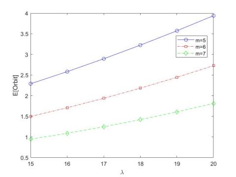
Figure 2. λ for various in m vs. E(Orbit)
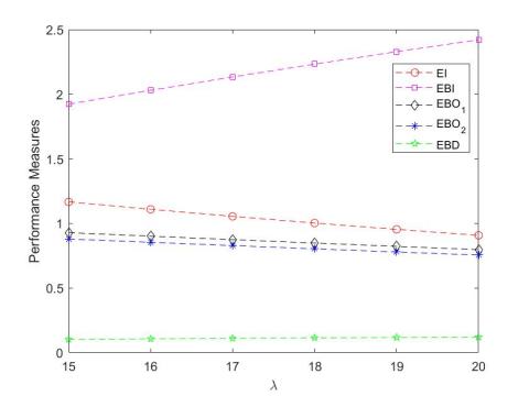
Figure 3. λ vs. Performance Measures
Case 1: For the following choices of parameters μ1=7, μ2=4, μ3=5, γ=5, r=0.7, η1=6, η2=7, α1=0.25, α2=0.1, α3=0.05, β1=3, β2=2, β3=1 and N=30, the outcomes resulting from variations in λ and m are portrayed in Figure 2. An escalation of the arrival rate of customer calls results in a proportional hike in the anticipated counts of orbital calls at the fiber optic customer care center. The Figure 3 demonstrates that a fixed value of m=5 results in a rise in the anticipated count of agents handling incoming calls and those vulnerable to breakdown, while the expected number of idle agents, agents handling outgoing calls and agents handling outgoing emails decreases with the rise in the arrival rate of customer calls.
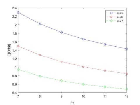
Figure 4. μ1 for various in m vs. E(Orbit)
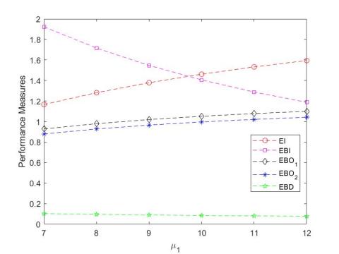
Figure 5. μ1 vs. Performance Measures
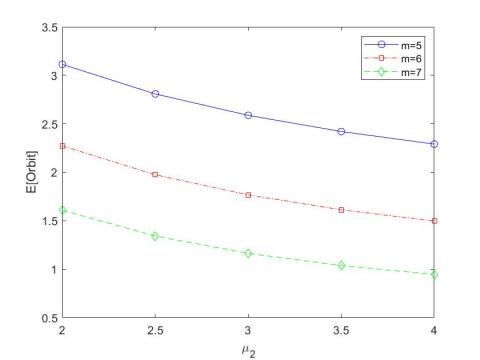
Figure 6. μ2 for various in m vs. E(Orbit)
Case 2: For λ=15, μ2=4, μ3=5, γ=5, r=0.7, η1=6, η2=7, α1=0.25, α2=0.1, α3=0.05, β1=3, β2=2, β3=1 and N=30, Figure 4 illustrates the outcomes resulting from variations in μ1 and m. Increasing the incoming call service rate μ1 results in a considerable decline in the anticipated count of orbital calls, regardless of the chosen value of m. Figure 5 shows that with a fixed value of m=5, a hike in μ1 results in a decline in the anticipated count of agents handling incoming calls and those susceptible to breakdown, while the expected number of idle agents, agents handling outgoing calls, and agents handling outgoing emails increases.
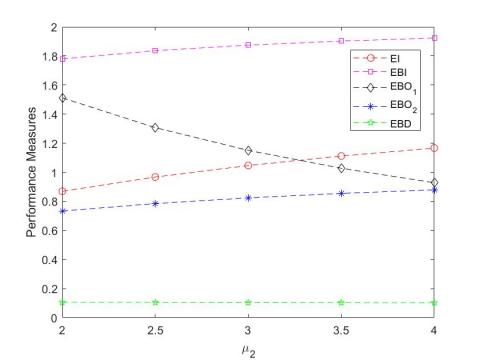
Figure 7. μ2 vs. Performance Measures
Case 3: By choosing λ=15, μ1=7, μ3=5, γ=5, r=0.7, η1=6, η2=7, α1=0.25, α2=0.1, α3=0.05, β1=3, β2=2, β3=1 and N=30, the effects of changing μ2 and m on system performance were investigated in Figure 6. Irrespective of the chosen value of m, increasing outgoing call service rate μ2 resulted in a reduction of the anticipated count of fiber optic customer care orbital calls. Moreover, the increase in μ2 with a fixed m=5 led to a decline in the anticipated count of agents handling outgoing calls and those susceptible to breakdown, but a hike in the anticipated count of idle agents, agents handling incoming calls, and agents handling outgoing emails, is depicted in Figure 7.
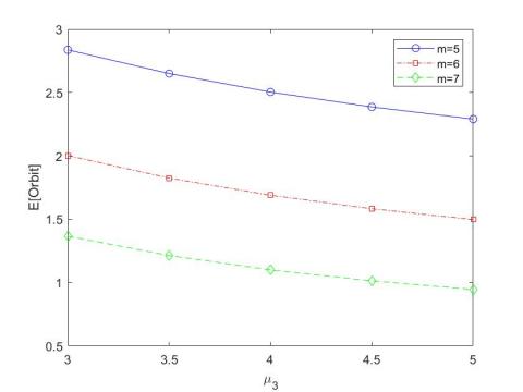
Figure 8. μ3 for various in m vs. E(Orbit)
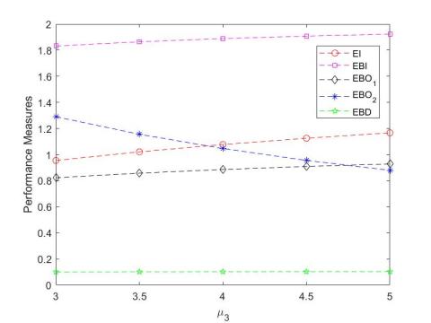
Case 4: The study was conducted on a system with λ=15, μ1=7, μ2=4, γ=5, r=0.7, η1=6, η2=7, α1=0.25, α2=0.1, α3=0.05, β1=3, β2=2, β3=1 and N=30. The impact of varying μ3 and m on system performance was investigated and presented in Figure 8. The results revealed that increasing outgoing email service rate μ3 led to a reduction in the anticipated count of fiber optic customer care calls waiting in the buffer, irrespective of the chosen value of m. Additionally, with a fixed m=5, a hike in μ3 resulted in a decline in the anticipated count of agents handling outgoing emails and those susceptible to breakdown, while increasing the expected number of idle agents, agents handling incoming calls, and agents handling outgoing calls, as illustrated in Figure 9.
Figure 9. μ3 vs. Performance Measures
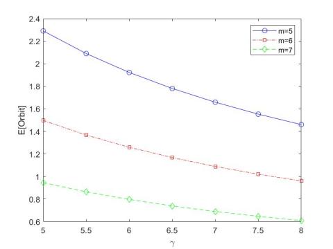
Figure 10. γ for various in m vs. E(Orbit)
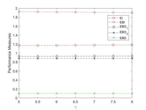
Figure 11. γ vs. Performance Measures
Case 5: Taking λ=15, μ1=7, μ2=4, μ3=5, r=0.7, η1=6, η2=7, α1=0.25, α2=0.1, α3=0.05, β1=3, β2=2, β3=1 and N=30. The results, presented in Figure 10, showed that increasing retrial incoming rate γ led to a decrease in the anticipated count of fiber optic customer care calls waiting in the buffer, regardless of the chosen m. Furthermore, when m=5, an increase in γ caused a reduction in the expected number of agents handling incoming calls and those at risk of breakdown, while increasing the expected number of idle agents, agents handling outgoing calls, and agents handling outgoing emails, as illustrated in Figure 11.
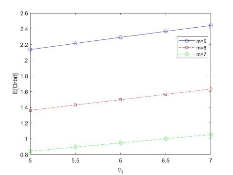
Figure 12. η1 for various in m vs. E(Orbit)
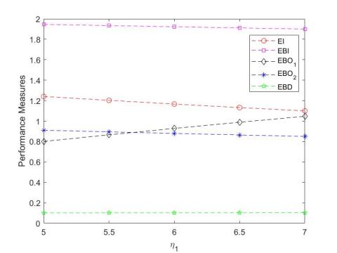
Case 6: The system performance was evaluated for λ=15, μ1=7, μ2=4, μ3=5, γ=5, r=0.7, η2=7, α1=0.25, α2=0.1, α3=0.05, β1=3, β2=2, β3=1 and N=30, and the outcomes are portrayed in Figure 12. It was noticed that increasing agents idle time before making outgoing calls rate η1 led to an increase in the anticipated count of fiber optic customer care calls waiting in the buffer, regardless of the chosen m. Moreover, when m=5, an increase in ${{\eta }_{1}}$ caused a reduction in the expected number of idle agents, agents busy handling incoming calls and agents handling outgoing emails, while increasing the expected number of agents handling outgoing calls and breakdown, as depicted in Figure 13.
Figure 13. η1 vs. Performance Measures
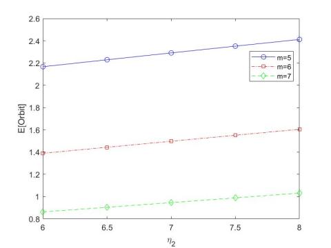
Figure 14. η2 for various in m vs. E(Orbit)
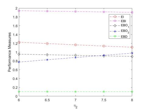
Case 7: For the given set of parameters, λ=15, μ1=7, μ2=4, μ3=5, γ=5, r=0.7, η1=6, α1=0.25, α2=0.1, α3=0.05, β1=3, β2=2, β3=1 and N=30, Figure 14 depicts the impact of varying agents idle time before sending outgoing emails rate η2 and m on the anticipated count of fiber optic customer care calls waiting in the buffer. It was observed that increasing η2 yields a corresponding rise in the anticipated count of calls waiting in the buffer, regardless of the chosen value of m. Furthermore, when m=5, an increase in η2 results in a reduction of the anticipated count of idle agents, agents occupied with incoming and outgoing calls, and agents susceptible to breakdown, while the expected number of agents handling outgoing emails increases, as presented in Figure 15.
Figure 15. η2 vs. Performance Measures
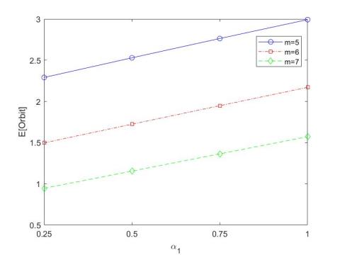
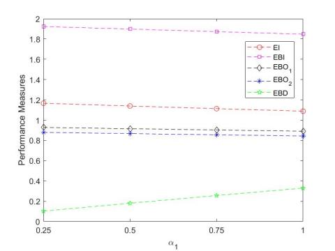
Case 8: The given parameters are λ=15, μ1=7, μ2=4, μ3=5, γ=5, r=0.7, η1=6, η2=7, α2=0.1, α3=0.05, β1=3, β2=2, β3=1 and N=30. Figure 16 shows the impact of varying rates of breakdown during incoming calls α1 and m on the anticipated count of fiber optic customer care orbital calls. The results indicate that increasing α1 results in a corresponding rise in the anticipated count of orbital calls, irrespective of the value of m. Moreover, when m=5, an increase in α1 causes a decline in the anticipated count of idle agents, agents handling incoming calls, outgoing calls and outgoing emails, while the expected number of agents susceptible to breakdown increases, as illustrated in Figure 17.
Figure 16. α1 for various in m vs. E(Orbit)
Figure 17. α1 vs. Performance Measures
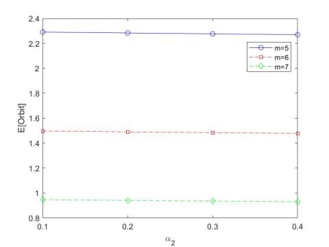
Figure 18. α2 for various in m vs. E(Orbit)
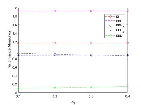
Case 9: Taking λ=15, μ1=7, μ2=4, μ3=5, γ=5, r=0.7, η1=6, η2=7, α1=0.25, α3=0.05, β1=3, β2=2, β3=1 and N=30. Figure 18 shows the impact of varying rates of breakdown during outgoing calls α2 and m on the anticipated count of fiber optic customer care orbital calls. The results indicate that increasing α2 results in a decline in the anticipated count of orbital calls, irrespective of the value of m. Moreover, when m=5, a rise in α2 yields in a hike in the anticipated count of idle agents, agents handling incoming calls, outgoing emails, and those susceptible to breakdown, while the expected number of agents handling outgoing calls decreases, as presented in Figure 19.
Figure 19. α2 vs. Performance Measures
Figure 20. α3 for various in m vs. E(Orbit)
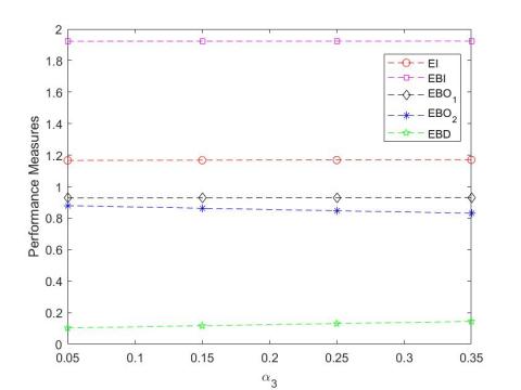
Figure 21. α3 vs. Performance Measures
Case 10: For the given parameters λ=15, μ1=7, μ2=4, μ3=5, γ=5, r=0.7, η1=6, η2=7, α1=0.25, α2=0.1, β1=3, β2=2, β3=1 and N=30, Figure 20 depicts the effect of varying rates of breakdown during outgoing emails α3 and m on the anticipated count of fiber optic customer care calls waiting in the buffer. It was observed that increasing α3 led to a decline in the anticipated count of orbital calls, regardless of the chosen value of m. Furthermore, when m=5, a rise in α3 yields in a hike in the anticipated count of idle agents, agents handling incoming and outgoing calls, and agents susceptible to breakdown, while the expected number of agents handling outgoing emails decreases, as presented in Figure 21.
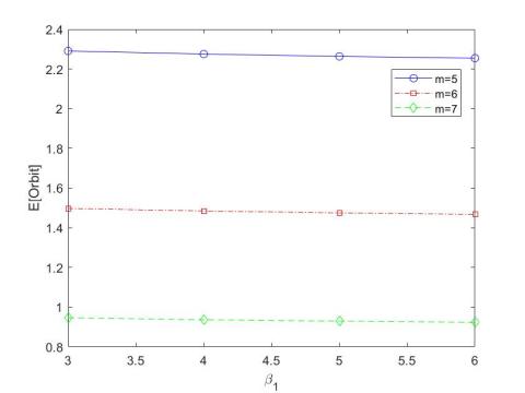
Figure 22. β1 for various in m vs. E(Orbit)
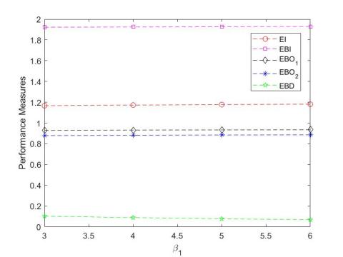
Case 11: For the given values of the parameters λ=15, μ1=7, μ2=4, μ3=5, γ=5, r=0.7, η1=6, η2=7, α1=0.25, α2=0.1, α3=0.05, β2=2, β3=1 and N=30, Figure 22 illustrates the effect of varying rates of repair during incoming calls β1 and m on the anticipated count of fiber optic customer care calls waiting in the buffer. It was observed that increasing β1 resulted in a corresponding decline in the anticipated count of orbital calls, regardless of the chosen value of m. Moreover, when m=5, an increase in β1 led to a hike in the anticipated count of idle agents, agents occupied with incoming and outgoing calls and outgoing emails, while the expected number of agents susceptible to breakdown decreased, as shown in Figure 23.
Figure 23. β1 vs. Performance Measures
Table 1 shows that as $\lambda$ increases, E[BI] and E[BD] increase while E[I], E[BO1] and E[BO2] decrease. Additionally, for varying values of $m$, an escalation in λ leads to a hike in E[Orbit]. The outcomes in Table 2 imply that increasing the value of μ1 leads to a decline in E[BI] and $E\left[ BD \right]$, while E[I], E[BO1] and E[BO2] increase. Moreover, for varying values of m, a hike in μ1 corresponds to a decline in E[Orbit]. Table 3 demonstrates that an increase in μ2 results in a negative correlation with E[BO1] and E[BD], but a positive correlation with E[I], E[BI] and E[BO2]. Additionally, there is an inverse relationship between an increase in μ2 and E[Orbit] for varying values of m. Table 4 shows that increasing ${{\mu }_{3}}$ is associated with a decrease in E[BO2] but an increase in E[I], E[BI], E[BO1] and E[BO2]. Furthermore, E[Orbit] declines with a hike in μ3 for different choices of m.
Table 5 presents that an increase in γ is inversely associated with E[BI] and E[BD] but positively associated with E[I], E[BO1] and E[BO2]. Furthermore, a hike in γ leads to a decline in the anticipated count E[Orbit] for varying values of m. Table 6 demonstrates that increasing η1 results in a decline in the expected values of E[I], E[BI] and E[BO2], while leading to an increase in E[BO1] and E[BD]. Moreover, an increase in η1 corresponds to an increase in the expected value of E[Orbit] for diverse values of m. Table 7 displays that an increase in η2 is inversely associated with the expected values of E[I], E[BI], E[BO1] and E[BD], but positively correlated with the expected value of E[BO2]. Additionally, a hike in η2 leads to an escalation in the anticipated value of E[Orbit] for varying values of $m$. Table 8 shows that increasing α1 results in a decrease in the expected values of E[I], E[BI], E[BO1] and E[BO2], while increasing the expected value of E[BD]. Moreover, an increase in α1 corresponds to an increase in the expected value of E[Orbit] for different values of m.
Table 1. Impact of λ on efficiency metrics for varying server count m
|
λ |
E[Orbit] |
E[I] |
E[BI] |
E[BO1] |
E[BO2] |
E[BD] |
||
|
m=5 |
m=6 |
m=7 |
||||||
|
15 |
2.2909 |
1.4973 |
0.9461 |
1.1666 |
1.9230 |
0.9283 |
0.8792 |
0.1029 |
|
16 |
2.5841 |
1.7089 |
1.0903 |
1.1090 |
2.0298 |
0.9010 |
0.8535 |
0.1067 |
|
17 |
2.8959 |
1.9377 |
1.2487 |
1.0543 |
2.1331 |
0.8742 |
0.8281 |
0.1103 |
|
18 |
3.2261 |
2.1838 |
1.4216 |
1.0026 |
2.2326 |
0.8479 |
0.8031 |
0.1139 |
|
19 |
3.5743 |
2.4473 |
1.6095 |
0.9536 |
2.3285 |
0.8220 |
0.7786 |
0.1172 |
|
20 |
3.9399 |
2.7284 |
1.8130 |
0.9074 |
2.4206 |
0.7968 |
0.7547 |
0.1204 |
Table 2. Impact of μ1 on efficiency metrics for varying server count m
|
μ1 |
E[Orbit] |
E[I] |
E[BI] |
E[BO1] |
E[BO2] |
E[BD] |
||
|
m=5 |
m=6 |
m=7 |
||||||
|
7 |
2.2909 |
1.4973 |
0.9461 |
1.1666 |
1.9230 |
0.9283 |
0.8792 |
0.1029 |
|
8 |
2.0241 |
1.2862 |
0.7912 |
1.2813 |
1.7163 |
0.9793 |
0.9276 |
0.0956 |
|
9 |
1.8215 |
1.1309 |
0.6802 |
1.3786 |
1.5468 |
1.0195 |
0.9657 |
0.0895 |
|
10 |
1.6638 |
1.0127 |
0.5975 |
1.4615 |
1.4061 |
1.0518 |
0.9962 |
0.0844 |
|
11 |
1.5380 |
0.9203 |
0.5339 |
1.5328 |
1.2879 |
1.0781 |
1.0212 |
0.0801 |
|
12 |
1.4358 |
0.8463 |
0.4836 |
1.5945 |
1.1874 |
1.0999 |
1.0418 |
0.0765 |
Table 3. Impact of μ2 on efficiency metrics for varying server count m
|
μ2 |
E[Orbit] |
E[I] |
E[BI] |
E[BO1] |
E[BO2] |
E[BD] |
||
|
m=5 |
m=6 |
m=7 |
||||||
|
2 |
3.1131 |
2.2727 |
1.6084 |
0.8695 |
1.7799 |
1.5117 |
0.7334 |
0.1055 |
|
2.5 |
2.8079 |
1.9749 |
1.3423 |
0.9672 |
1.8360 |
1.3069 |
0.7850 |
0.1048 |
|
3 |
2.5871 |
1.7663 |
1.1641 |
1.0464 |
1.8745 |
1.1508 |
0.8241 |
0.1042 |
|
3.5 |
2.4205 |
1.6134 |
1.0384 |
1.1118 |
1.9022 |
1.0277 |
0.8547 |
0.1035 |
|
4 |
2.2909 |
1.4973 |
0.9461 |
1.1666 |
1.9230 |
0.9283 |
0.8792 |
0.1029 |
Table 4. Impact of μ3 on efficiency metrics for varying server count m
|
μ3 |
E[Orbit] |
E[I] |
E[BI] |
E[BO1] |
E[BO2] |
E[BD] |
||
|
m=5 |
m=6 |
m=7 |
||||||
|
3 |
2.8370 |
2.0026 |
1.3666 |
0.9548 |
1.8318 |
0.8226 |
1.2901 |
0.1008 |
|
3.5 |
2.6502 |
1.8250 |
1.2136 |
1.0211 |
1.8644 |
0.8575 |
1.1554 |
0.1016 |
|
4 |
2.5040 |
1.6894 |
1.1004 |
1.0771 |
1.8889 |
0.8857 |
1.0461 |
0.1022 |
|
4.5 |
2.3868 |
1.5828 |
1.0139 |
1.1251 |
1.9079 |
0.9089 |
0.9555 |
0.1026 |
|
5 |
2.2909 |
1.4973 |
0.9461 |
1.1666 |
1.9230 |
0.9283 |
0.8792 |
0.1029 |
Table 5. Impact of γ on efficiency metrics for varying server count m
|
γ |
E[Orbit] |
E[I] |
E[BI] |
E[BO1] |
E[BO2] |
E[BD] |
||
|
m=5 |
m=6 |
m=7 |
||||||
|
5 |
2.2909 |
1.4973 |
0.9461 |
1.1666 |
1.9230 |
0.9283 |
0.8792 |
0.1029 |
|
5.5 |
2.0901 |
1.3679 |
0.8651 |
1.1694 |
1.9192 |
0.9289 |
0.8798 |
0.1028 |
|
6 |
1.9226 |
1.2598 |
0.7974 |
1.1722 |
1.9154 |
0.9294 |
0.8804 |
0.1026 |
|
6.5 |
1.7807 |
1.1682 |
0.7401 |
1.1748 |
1.9118 |
0.9300 |
0.8809 |
0.1025 |
|
7 |
1.6589 |
1.0896 |
0.6908 |
1.1774 |
1.9082 |
0.9306 |
0.8814 |
0.1024 |
|
7.5 |
1.5533 |
1.0212 |
0.6479 |
1.1799 |
1.9047 |
0.9311 |
0.8820 |
0.1022 |
|
8 |
1.4606 |
0.9613 |
0.6103 |
1.1824 |
1.9014 |
0.9317 |
0.8825 |
0.1021 |
Table 6. Impact of η1 on efficiency metrics for varying server count m
|
η1 |
E[Orbit] |
E[I] |
E[BI] |
E[BO1] |
E[BO2] |
E[BD] |
||
|
m=5 |
m=6 |
m=7 |
||||||
|
5 |
2.1356 |
1.3623 |
0.8422 |
1.2409 |
1.9458 |
0.8009 |
0.9104 |
0.1020 |
|
5.5 |
2.2138 |
1.4298 |
0.8936 |
1.2028 |
1.9344 |
0.8658 |
0.8946 |
0.1025 |
|
6 |
2.2909 |
1.4973 |
0.9461 |
1.1666 |
1.9230 |
0.9283 |
0.8792 |
0.1029 |
|
6.5 |
2.3667 |
1.5647 |
0.9994 |
1.1322 |
1.9116 |
0.9885 |
0.8643 |
0.1033 |
|
7 |
2.4413 |
1.6319 |
1.0534 |
1.0997 |
1.9001 |
1.0467 |
0.8498 |
0.1037 |
Table 7. Impact of η2 on efficiency metrics for varying server count m
|
η2 |
E[Orbit] |
E[I] |
E[BI] |
E[BO1] |
E[BO2] |
E[BD] |
||
|
m=5 |
m=6 |
m=7 |
||||||
|
6 |
2.1670 |
1.3893 |
0.8626 |
1.2261 |
1.9410 |
0.9546 |
0.7750 |
0.1032 |
|
6.5 |
2.2293 |
1.4433 |
0.9040 |
1.1957 |
1.9320 |
0.9413 |
0.8279 |
0.1031 |
|
7 |
2.2909 |
1.4973 |
0.9461 |
1.1666 |
1.9230 |
0.9283 |
0.8792 |
0.1029 |
|
7.5 |
2.3517 |
1.5512 |
0.9886 |
1.1387 |
1.9140 |
0.9155 |
0.9291 |
0.1027 |
|
8 |
2.4117 |
1.6050 |
1.0317 |
1.1119 |
1.9049 |
0.9031 |
0.9776 |
0.1026 |
Table 8. Impact of α1 on efficiency metrics for varying server count m
|
α1 |
E[Orbit] |
E[I] |
E[BI] |
E[BO1] |
E[BO2] |
E[BD] |
||
|
m=5 |
m=6 |
m=7 |
||||||
|
0.25 |
2.2909 |
1.4973 |
0.9461 |
1.1666 |
1.9230 |
0.9283 |
0.8792 |
0.1029 |
|
0.5 |
2.5294 |
1.7238 |
1.1550 |
1.1392 |
1.8980 |
0.9153 |
0.8669 |
0.1806 |
|
0.75 |
2.7635 |
1.9486 |
1.3639 |
1.1132 |
1.8728 |
0.9027 |
0.8551 |
0.2563 |
|
1 |
2.9930 |
2.1713 |
1.5726 |
1.0885 |
1.8474 |
0.8907 |
0.8436 |
0.3298 |
Table 9. Impact of α2 on efficiency metrics for varying server count m
|
α2 |
E[Orbit] |
E[I] |
E[BI] |
E[BO1] |
E[BO2] |
E[BD] |
||
|
m=5 |
m=6 |
m=7 |
||||||
|
0.1 |
2.2909 |
1.4973 |
0.9461 |
1.1666 |
1.9230 |
0.9283 |
0.8792 |
0.1029 |
|
0.2 |
2.2834 |
1.4906 |
0.9409 |
1.1698 |
1.9242 |
0.9076 |
0.8807 |
0.1178 |
|
0.3 |
2.2762 |
1.4843 |
0.9359 |
1.1728 |
1.9254 |
0.8879 |
0.8820 |
0.1320 |
|
0.4 |
2.2694 |
1.4783 |
0.9312 |
1.1757 |
1.9265 |
0.8690 |
0.8833 |
0.1456 |
Table 10. Impact of α3 on efficiency metrics for varying server count m
|
α3 |
E[Orbit] |
E[I] |
E[BI] |
E[BO1] |
E[BO2] |
E[BD] |
||
|
m=5 |
m=6 |
m=7 |
||||||
|
0.05 |
2.2909 |
1.4973 |
0.9461 |
1.1666 |
1.9230 |
0.9283 |
0.8792 |
0.1029 |
|
0.15 |
2.2880 |
1.4947 |
0.9441 |
1.1678 |
1.9235 |
0.9288 |
0.8627 |
0.1172 |
|
0.25 |
2.2852 |
1.4923 |
0.9421 |
1.1690 |
1.9239 |
0.9294 |
0.8468 |
0.1309 |
|
0.35 |
2.2826 |
1.4899 |
0.9403 |
1.1701 |
1.9243 |
0.9299 |
0.8314 |
0.1442 |
Table 11. Impact of β1 efficiency metrics for varying server count m
|
β1 |
E[Orbit] |
E[I] |
E[BI] |
E[BO1] |
E[BO2] |
E[BD] |
||
|
m=5 |
m=6 |
m=7 |
||||||
|
3 |
2.2909 |
1.4973 |
0.9461 |
1.1666 |
1.9230 |
0.9283 |
0.8792 |
0.1029 |
|
4 |
2.2753 |
1.4845 |
0.9366 |
1.1727 |
1.9257 |
0.9312 |
0.8820 |
0.0884 |
|
5 |
2.2637 |
1.4750 |
0.9295 |
1.1773 |
1.9276 |
0.9334 |
0.8842 |
0.0774 |
|
6 |
2.2546 |
1.4676 |
0.9240 |
1.1810 |
1.9292 |
0.9352 |
0.8858 |
0.0689 |
Table 9 demonstrates that an increase in α2 is associated with a decrease in the expected value of E[Orbit] for varying values of m. This increase in α2 also results in an escalation in the anticipated values of E[I], E[BI], E[BO2] and E[BD], while causing a decrease in the expected value of E[BO1]. Table 10 shows that increasing α3 results in higher expected values of E[I], E[BI], E[BO1] and E[BD], but lower expected value of E[BO2]. In addition, a hike in α3 causes a decline in E[Orbit] for various $m$ values. The results in Table 11 demonstrate that increasing the values of β1 results in a hike in the anticipated values of E[I], E[BI], E[BO1] and E[BO2], while decreasing the expected value of E[BD]. Additionally, for varying values of m, a hike in β1 corresponds to a decline in the expected value of E[Orbit].
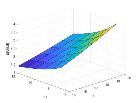
Figure 24. λ vs. μ1 vs. E(Orbit)
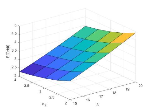
Three-dimensional graphical representations are utilized to explore how alterations in system parameters influence overall system performance. The anticipated count of orbital calls at the fiber optic customer care centre E[Orbit] rises with a hike in the rate of arrival λ and decline with an escalation in the incoming call μ1 as portrayed in Figure 24. Figure 25 conveys that an escalation in the arrival rate λ causes a rise in the anticipated count of incoming orbital calls E[Orbit], whereas a hike in outgoing call μ2 brings about a decrease in E[Orbit].
Figure 25. λ vs. μ2 vs. E(Orbit)
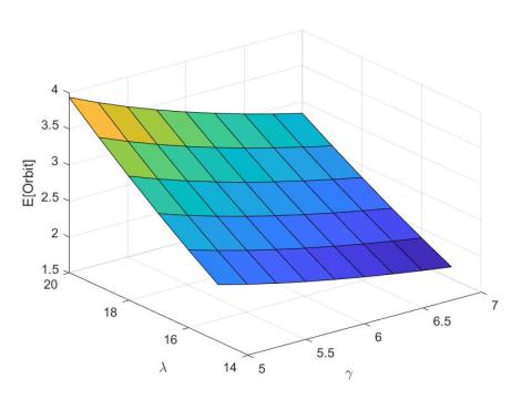
Figure 26. γ vs. λ vs. E(Orbit)
Figure 26 interprets that an escalation in the arrival rate λ causes a hike in the anticipated count of orbital calls E[Orbit], whereas a hike in retrial rate γ brings about a decrease in E[Orbit].
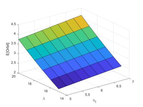
Figure 27. η1 vs. λ vs. E(Orbit)
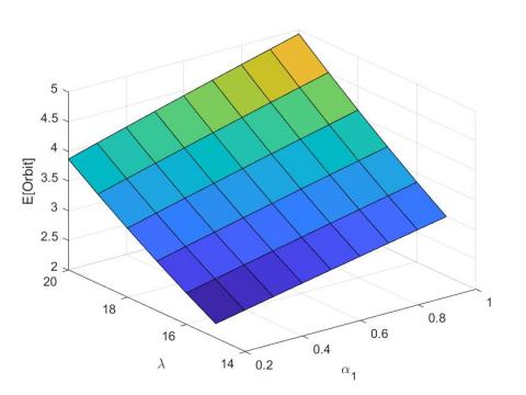
Figure 28. α1 vs. λ vs. E(Orbit)
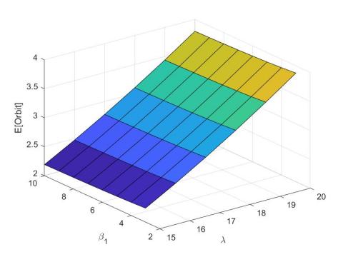
Figure 29. λ vs. β1 vs. E(Orbit)
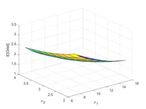
Rise in E(Orbit) is noted with a hike in the making outgoing call rate η1 and a rise in the same is witnessed with a hike in the λ of orbital customers is clear from Figure 27. The anticipated count of orbital calls at the fiber optic care E(Orbit) rises with a hike in λ and escalates with a rise in the α1 as shown in Figure 28. The anticipated count of orbital calls at the fiber optic customer care centre E(Orbit) rises with a hike in λ and decreases with a hike in the β1 as portrayed in Figure 29. The anticipated count of incoming orbital calls at fiber optic customer care centre E(Orbit) reduces with a rise in incoming call service rate μ1 and reduces with a rise in the outgoing call service rate μ2 as shown in Figure 30.
Figure 30. μ1 vs. μ2 vs. E(Orbit)
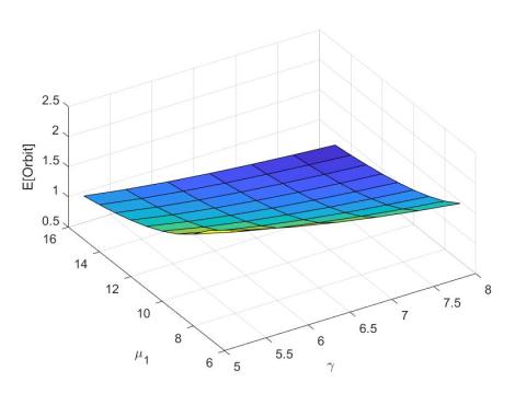
Figure 31. γ vs. μ1 vs. E(Orbit)
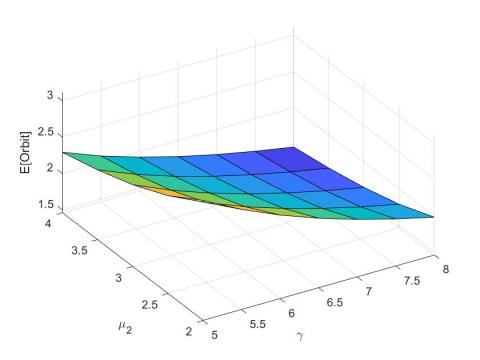
Figure 32. γ vs. μ2 vs. E(Orbit)
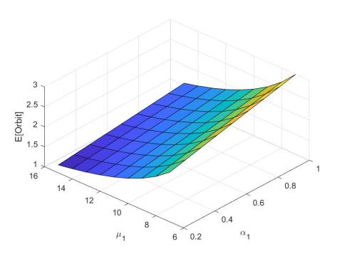
The anticipated count of orbital calls at the fiber optic customer care centre E(Orbit) reduces with a rise in retrial rate γ and reduces with a rise in incoming call service rate μ1 as portrayed in Figure 31. It is evident from Figure 32 that a hike in the retrial rate γ brings about a decrease in the anticipated count of orbital calls E(Orbit), whereas a hike in outgoing call service rate μ1 brings about a decrease in E(Orbit). The plot in Figure 33 portrays an increase in the anticipated count of orbital calls at the fiber optic customer care centre E(Orbit) for a hike in breakdown rate α1 during incoming calls and decreasing trend for a hike in the incoming call service rate μ1.
Figure 33. α1 vs. μ1 vs. E(Orbit)
From the numerical investigation, we infer that for enhancing the efficiency of the proposed model, an increase in the service provision rates of incoming calls, outgoing calls and emails, retrial call rates and repair rates is beneficial. In addition, minimising the duration of idle times before making outgoing services serves effective in the improvement of the system efficiency. At the same time controlling the breakdown rates has a good impact on reducing the likely chances of potential reneging of customers. Moreover, higher arrival rates call for an increase in the number of agents.
The current study examines a multiple server retrial queue with unreliable servers, reneging and two types of outgoing services. Using QBD process, we have derived the stability condition essential for the existence of steady state probabilities. The equilibrium probabilities of the system size distribution are calculated using the MGM and several efficiency metrics are evaluated to assess the performance of the proposed model. The model is illustrated with a brief example of a fiber optic customer care center. This work investigates the influence of varying system based parameters on the efficiency measures, which are visually presented through numerical and graphical illustrations. Moreover, the inference drawn from numerical investigation is also interpreted in context of the practical implementation of variations in system parameters, associated with fibre optic customer care center. This work can be further explored on retrial queues with working breakdown and working vacation.
The authors wish to express their appreciation to the Editorial board and referees for their invaluable insights and suggestions, which have significantly improved the quality of the initial manuscript.
[1] Dutta, K., Choudhury, A. (2020). Estimation of performance measures of M/M/1 queues–a simulation-based approach. International Journal of Applied Management Science, 12(4): 265-279. https://doi.org/10.1504/IJAMS.2020.110346
[2] Kim, J., Kim, B. (2016). A survey of retrial queueing systems. Annals of Operations Research, 247: 3-36. https://doi.org/10.1007/s10479-015-2038-7
[3] Zhang, X., Wang, J., Ma, Q. (2017). Optimal design for a retrial queueing system with state-dependent service rate. Journal of Systems Science and Complexity, 30(4): 883-900. https://doi.org/10.1007/s11424-017-5097-9
[4] Moiseev, A., Nazarov, A., Paul, S. (2020). Asymptotic diffusion analysis of multi-server retrial queue with hyper-exponential service. Mathematics, 8(4): 531. https://doi.org/10.3390/math8040531
[5] Fiems, D. (2022). Retrial queues with generally distributed retrial times. Queueing Systems, 100(3-4): 189-191. https://doi.org/10.1007/s11134-022-09793-4
[6] Arivudainambi, D., Godhandaraman, P. (2015). Retrial queueing system with balking, optional service and vacation. Annals of Operations Research, 229: 67-84. https://doi.org/10.1007/s10479-014-1765-5
[7] Ding, D., Ou, J., Ang, J. (2015). Analysis of ticket queues with reneging customers. Journal of the Operational Research Society, 66(2): 231-246. https://doi.org/10.1057/jors.2013.185
[8] Singh, C.J., Jain, M., Kumar, B. (2016). Analysis of single server finite queueing model with reneging. International Journal of Mathematics in Operational Research, 9(1): 15-38. https://doi.org/10.1504/IJMOR.2016.077558
[9] Wang, Q., Zhang, B. (2018). Analysis of a busy period queuing system with balking, reneging and motivating. Applied Mathematical Modelling, 64: 480-488. https://doi.org/10.1016/j.apm.2018.07.053
[10] Chang, J., Wang, J. (2018). Unreliable M/M/1/1 retrial queues with set-up time. Quality Technology & Quantitative Management, 15(5): 589-601. https://doi.org/10.1080/16843703.2017.1320459
[11] Kuki, A., Bérczes, T., Sztrik, J., Kvach, A. (2019). Numerical analysis of retrial queueing systems with conflict of customers and an unreliable server. Journal of Mathematical Sciences, 237: 673-683. https://doi.org/10.1007/s10958-019-04193-1
[12] Atencia, I., Galán-García, J.L. (2021). Sojourn times in a queueing system with breakdowns and general retrial times. Mathematics, 9(22): 2882. https://doi.org/10.3390/math9222882
[13] Liu, T.H., Chang, F.M., Ke, J.C., Sheu, S.H. (2022). Optimization of retrial queue with unreliable servers subject to imperfect coverage and reboot delay. Quality Technology & Quantitative Management, 19(4): 428-453. https://doi.org/10.1080/16843703.2021.2020952
[14] Poongothai, V., Saravanan, V., Kannan, M., Godhandaraman, P. (2022). An M/M/2 retrial queueing system with discouragement, breakdowns and repairs. In AIP Conference Proceedings, 2516(1): 360010. https://doi.org/10.1063/5.0109027
[15] Saravanan, V., Poongothai, V., Godhandaraman, P. (2023). Admission control policy of a two heterogeneous server finite capacity retrial queueing system with maintenance activity. Opsearch, 1-24. https://doi.org/10.1007/s12597-023-00669-6
[16] Yiming, N., Guo, B. Z. (2023). Asymptotic behavior of a retrial queueing system with server breakdowns. Journal of Mathematical Analysis and Applications, 520(1): 126867. https://doi.org/10.1016/j.jmaa.2022.126867
[17] Saravanan, V., Poongothai, V., Godhandaraman, P. (2023). Performance analysis of a retrial queueing system with optional service, unreliable server, balking and feedback. International Journal of Mathematical, Engineering and Management Sciences, 8(4): 769-786. https://doi.org/10.33889/IJMEMS.2023.8.4.044
[18] Yang, D.Y., Ke, J.C., Wu, C.H. (2015). The multi-server retrial system with Bernoulli feedback and starting failures. International Journal of Computer Mathematics, 92(5): 954-969. https://doi.org/10.1080/00207160.2014.932908
[19] Chang, F.M., Liu, T.H., Ke, J.C. (2018). On an unreliable-server retrial queue with customer feedback and impatience. Applied Mathematical Modelling, 55: 171-182. https://doi.org/10.1016/j.apm.2017.10.025
[20] Ke, J.C., Liu, T.H., Su, S., Zhang, Z.G. (2022). On retrial queue with customer balking and feedback subject to server breakdowns. Communications in Statistics-Theory and Methods, 51(17): 6049-6063. https://doi.org/10.1080/03610926.2020.1852432
[21] Saravanan, V., Poongothai, V., Godhandaraman, P. (2023). Performance analysis of a multi server retrial queueing system with unreliable server, discouragement and vacation model. Mathematics and Computers in Simulation, 214, 204-226. https://doi.org/10.1016/j.matcom.2023.07.008
[22] Artalejo, J.R., Phung-Duc, T. (2013). Single server retrial queues with two way communication. Applied Mathematical Modelling, 37(4): 1811-1822. https://doi.org/10.1016/j.apm.2012.04.022
[23] Phung-Duc, T., Rogiest, W., Takahashi, Y., Bruneel, H. (2016). Retrial queues with balanced call blending: analysis of single-server and multiserver model. Annals of Operations Research, 239: 429-449. https://doi.org/10.1007/s10479-014-1598-2
[24] Sakurai, H., Phung-Duc, T. (2016). Scaling limits for single server retrial queues with two-way communication. Annals of Operations Research, 247: 229-256. https://doi.org/10.1007/s10479-015-1874-9
[25] Kumar, M.S., Dadlani, A., Kim, K. (2020). Performance analysis of an unreliable M/G/1 retrial queue with two-way communication. Operational Research, 20: 2267-2280. https://doi.org/10.1007/s12351-018-0417-y
[26] Neuts, M.F. (1994). Matrix-geometric Solutions in Stochastic Models: An Algorithmic Approach. Courier Corporation.
[27] Latouche, G., Ramaswami, V. (1999). Introduction to matrix analytic methods in stochastic modeling. Society for Industrial and Applied Mathematics.