Optimizing Two-Warehouse Inventory for Shelf-Life Stock with Time-Varying Bi-Quadratic Demand Under Shortages and Inflation

A successful business must effectively manage its inventory, and this is especially crucial when it comes to goods that are deteriorating. But managing deteriorating inventory can be difficult since there are so many things to take into account, including shifts in demand, holding costs, backlogs, shortages, and inflation. Numerous researchers have created models that attempt to optimise inventory management for degrading items by taking into consideration these issues in response to these difficulties.

Mishra and Singh [1] employed a computational approach to optimize the total cost function of an inventory model that accounts for ramp-type demand and linear deterioration. Venkateswarlu and Mohan [2] developed a deterministic inventory model for deteriorating items that integrates quadratic demand functions and proportional deterioration rates. Meanwhile, Chauhan and Singh [3] investigated optimal replenishment and ordering policies for time-varying deterioration items with varying demand, utilizing a discounted cash flow approach.

A model for calculating the Economic Order Quantity (EOQ) for non-instantaneously deteriorating items with stock-dependent demand, inflation, and partial backlogging was introduced by Palanivel et al. [4], which utilizes two warehouses. In a separate study, Kumar and Chanda [5] presented a two-warehouse inventory model specifically designed for technology products. Yadav and Swami [6] developed a model for non-instantaneous deteriorating items that considers rented and owned warehouses.

Shaikh et al. [7] suggested a two-warehouse inventory model that considers partial backlogging and advanced payment. Taghizadeh-Yazdi et al. [8] proposed a mathematical programming model that maximizes the profit of suppliers, manufacturers, and distributors in a three-echelon supply chain, accounting for the deteriorating nature of raw materials and final products. Meanwhile, Khan et al. [9] presented a two-storage inventory model with advance payment, where demand is dependent on the selling price. The model also takes into account partial shortages with a fixed backlogging rate.

Mashud [10] proposed an Economic Order Quantity (EOQ) inventory model that considers deteriorating items with stock-dependent demand and full backlogged shortages, while also taking into account price changes. Suman [11] presented a deterministic inventory model for deteriorating items with a biquadratic demand function over time and allowing for shortages. A strategy where suppliers give price discounts to retailers that make advance payments was presented in Duary et al. 's [12] study.

The review focuses on the problems that companies run into while trying to manage deteriorating inventories and the models that have been put out in various studies to solve these problems. By taking into account elements like demand volatility, holding costs, backlogs, shortages, and inflation, these models can aid in the optimisation of inventory decisions. These research' conclusions offer useful information about how to manage inventory for degrading goods, which can aid firms in making wise choices. In light of the effects of price variations on overall profit, recent researches have proposed novel models to manage supply chains with uncertain demand and inflation. Businesses can benefit from extra advice from the three-level supply chain model by Padiyar et al. [13] and the Stackelberg game-based model by Mahdavisharif et al. [14] to increase their inventory management and general profitability. The literature review provided corresponds to the data presented in Table 1.

While some prior research has considered shelf-life goods in inventory management models, there remains a research gap in the development of comprehensive inventory models tailored specifically to address the intricate challenges posed by these goods. The existing literature may have touched on aspects of shelf-life management, but opportunities exist to refine and expand these models further. This research aims to bridge this gap by presenting an advanced and holistic inventory model that comprehensively accounts for factors specific to goods with a limited shelf life, such as biquadratic time-dependent demand, inflation, and partial backlogged shortages.

The motivation behind this research is deeply rooted in the pressing need for efficient inventory management tailored specifically to goods characterized by a limited shelf life. Effectively managing these products poses a complex challenge, one that involves the careful consideration of several crucial cost components, namely holding cost, deterioration cost, shortage cost, and lost sale cost.

At its core, the primary aim of this research is to craft a comprehensive inventory model meticulously designed to optimize the replenishment strategy for shelf-life goods, all while intricately addressing these fundamental cost elements. The ultimate aspiration is to provide invaluable assistance to companies in making judicious inventory decisions, ultimately culminating in the minimization of these indispensable costs.

This research introduces a novel inventory model meticulously crafted to enhance the replenishment plan for products subjected to the constraints of a limited shelf life. It meticulously factors in a spectrum of variables, including the intricacies of biquadratic time-dependent demand, the influence of inflation, and the implications of partial backlogged shortages. The paramount significance of this work lies in its profound ability to amalgamate these critical components into a unified and comprehensive model. In stark contrast to prior studies, which often scrutinized these factors in isolation, this research takes on a holistic perspective.

One of the most compelling advantages inherent in the adoption of this model lies in its transformative capacity to guide companies in making well-considered inventory decisions, subsequently leading to the minimization of operational costs and the overarching enhancement of organizational efficiency.

Table 1. Literature review for the proposed model

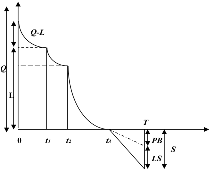
The objective of this model formulation is to analyze the inventory management system of a warehouse that stores a lot size of Q units. Among the Q units, L units are placed in an owned warehouse, and the remaining Q-L units are placed in a rented warehouse. The rented warehouse depletes due to demand only, as the product has a shelf-life, and becomes zero during the time period [0 t₁]. On the other hand, the owned warehouse remains constant during this period.

During the time interval [t₁ t₂], the owned warehouse starts depleting due to demand only. After this period, during the time interval [t₂ t₃], the owned warehouse becomes zero due to the combined effect of deterioration and demand. Subsequently, during the time period [t₃ T], shortages occur, and the level of negative inventory during this time interval is represented by I_s(t).

161.png

Figure 1. Graphical representation of the proposed two-warehouse inventory model

To better understand the behaviour of this inventory management system over the time interval [0 T], a graphical representation has been provided in Figure 1. This model formulation takes into account various factors such as inventory level, demand, deterioration, and shortage to provide a comprehensive view of the inventory management system of the warehouse.

The governing differential equations for above inventory model are represented by:

$\frac{d{{I}_{r}}\left( t \right)}{dt}=-D\left( t \right)\text{, 0}<t\le {{t}_{1}}$      (1)

$\frac{d{{I}_{o}}\left( t \right)}{dt}=-D\left( t \right)\text{,  }{{t}_{1}}\le t\le {{t}_{2}}$      (2)

$\frac{d{{I}_{o}}\left( t \right)}{dt}+\zeta {{I}_{o}}\left( t \right)=-D\left( t \right)\text{,  }{{t}_{2}}\le t\le {{t}_{3}}$      (3)

$\frac{d{{I}_{s}}\left( t \right)}{dt}=-D\left( t \right)\Upsilon \text{,  }{{t}_{3}}\le t\le T$      (4)

The solutions to the aforementioned differential equation, determined by applying the specified boundary conditions I_r(t₁)=0, I_o(t₁)=L, I_o(t₃)=0, I_s(t₃)=0 respectively, are as follows:

${{I}_{r}}\left( t \right)=\frac{\beta t_{1}^{5}}{5}+\alpha \left( {{t}_{1}}-t \right)-\frac{\beta {{t}^{5}}}{5}\text{,  0}<t\le {{t}_{1}}$      (5)

${{I}_{o}}\left( t \right)=\frac{\beta t_{1}^{5}}{5}+\alpha {{t}_{1}}+L-\alpha t-\frac{\beta {{t}^{5}}}{5}\text{,  }{{t}_{1}}\le t\le {{t}_{2}}$      (6)

$\begin{aligned} & I_o(t)=\left[\begin{array}{l}\frac{e^{-\zeta\left(t-t_3\right)}\left(\beta \zeta^4 t_3^4+\alpha \zeta^4-4 \beta \zeta^3 t_3^3+12 \beta \zeta^2 t_2^2-24 \beta \zeta t_3+24 \beta\right)}{\zeta^5} \\ -\frac{\left(\alpha \zeta^4+24 \beta\right)}{\zeta^5}-\frac{\beta t^4}{\zeta}+\frac{4 \beta t^3}{\zeta^2}-\frac{12 \beta t^2}{\zeta^3}+\frac{24 \beta t}{\zeta^4}\end{array}\right], \\ & t_2 \leq \mathrm{t} \leq t_3\end{aligned}$      (7)

${{I}_{s}}\left( t \right)=-\alpha \Upsilon \left( t-{{t}_{\text{3}}} \right)\text{,  }{{t}_{3}}\le t\le T$      (8)

By considering continuity at time t=t₂in the OW, it can be deduced from Eqs. (6) and (7) that:

$L=\left[\begin{array}{l}\alpha t_2-\alpha t_1-\frac{\beta t_2^4}{\zeta}+\frac{4 \beta t_2^3}{\zeta^2}-\frac{12 \beta t_2^2}{\zeta^3}+\frac{24 \beta t_2}{\zeta^4} \\ -\frac{\alpha \zeta^4+24 \beta}{\zeta^5}-\frac{\beta t_1^5}{5}+\frac{\beta t_2^5}{5}+ \\ \frac{e^{-\zeta\left(t_2-t_3\right)}\left(\beta \zeta^4 t_3^4+\alpha \zeta^4-4 \beta \zeta^3 t_3^3+12 \beta \zeta^2 t_3^2-24 \beta \zeta t_3+24 \beta\right)}{\zeta^5}\end{array}\right]$      (9)

In the context of RW, there exists a quantity Q-L unit at the initial time t. To calculate the value of Q-L and putting the value of t=0 in the (5). we get:

${{I}_{r}}\left( 0 \right)=Q-L=\frac{\beta t_{1}^{5}}{5}+\alpha {{t}_{1}}$

Furthermore, by substituting t=T into Eq. (8), we can determine the maximum level of backlogging that occurs per cycle, i.e. S=-αϒ(T-t₃).

Hence, the total quantity to be replenished per cycle can be expressed as follows: TQC=Q-S.

$T Q C=\left[\begin{array}{l}\frac{e^{-\zeta\left(t_2-t_3\right)}\left(\begin{array}{l}\beta \zeta^4 t_3^4+\alpha \zeta^4-4 \beta \zeta^3 t_3^3 \\ +12 \beta \zeta^2 t_3^2-24 \beta \zeta t_3+24 \beta\end{array}\right)}{\zeta^5} \\ +\frac{4 \beta t_2^3}{\zeta^2}-\frac{12 \beta t_2^2}{\zeta^3}+\frac{24 \beta t_2}{\zeta^4}-\frac{\alpha \zeta^4+24 \beta}{\zeta^5} \\ -\frac{\beta t_1^5}{5}+\frac{\beta t_2^5}{5}+\frac{\beta t_1^5}{5}+\alpha t_1+\alpha \Upsilon\left(T-t_3\right) \\ -\frac{\beta t_2^4}{\zeta}+\alpha t_2-\alpha t_1\end{array}\right]$      (10)

The total cost per cycle comprises the following components:

I. Ordering cost per cycle

$O C=A$

II. Inventory holding cost per cycle in the R.W

$H C_{r w}=H_1 \int_0^{t_1} I_r(t) e^{-r t} d t$

$H C_{r w}=\frac{H_1 e^{-r t_1}}{5 r^6}\left[\begin{array}{l}120 \beta-120 \beta e^{r t_1}+5 \alpha r^4-5 \alpha r^4 e^{r t_1} \\ +60 \beta r^2 t_1^2+20 \beta r^3 t_1^3+5 \beta r^4 t_1^4+ \\ 120 \beta r t_1+\beta r^5 t_1^5 e^{r t_1}+5 \alpha r^5 t_1 e^{r t_1}\end{array}\right]$

III. The inventory holding cost per cycle in OW

$H C_{o w}=H_2 \int_0^{t_3} I_o(t) e^{-r t} d t$

$H C_{o w}=H_2\left[\int_0^{t_1} I_o(t) e^{-r t} d t+\int_{t_1}^{t_2} I_o(t) e^{-r t} d t+\int_{t_2}^{t_3} I_o(t) e^{-r t} d t\right]$

$H C_{\text {ow }}=-H_2\left\{\begin{array}{l}{\begin{aligned} & \frac{\alpha\left(e^{-r t_1}\left(r t_1+1\right)-e^{-r t_2}\left(r t_2+1\right)\right)}{r^2}+\frac{\beta}{5}\left[\begin{aligned}

& \frac{e^{-r t_1}\left(r^5 t_1^5+5 r^4 t_1^4+20 r^3 t_1^3+60 r^2 t_1^2+120 r t_1+120\right)}{r^6} \\

& -\frac{e^{-r t_2}\left(r^5 t_2^5+5 r^4 t_2^4+20 r^3 t_2^3+60 r^2 t_2^2+120 r t_2+120\right)}{r^6}

\end{aligned}\right] \\ & -\frac{L\left(e^{-r t_1}-e^{-r t_2}\right)}{r}-\frac{24 \beta}{\zeta^4}\left[\frac{e^{-r t_2}\left(r t_2+1\right)-e^{-r t_3}\left(r t_3+1\right)}{r^2}\right]+\frac{12 \beta}{\zeta^3}\left[\begin{aligned}

& e^{-r t_2}\left(r^2 t_2^2+2 r t_2+2\right) \\

& \frac{-e^{-r t_3}\left(r^2 t_3^2+2 r t_3+2\right)}{r^3}

\end{aligned}\right] \\ & \end{aligned}} \\ {\begin{aligned} & -\frac{4 \beta}{\zeta^2}\left[\frac{e^{-r_2}\left(r^3 t_2^3+3 r^2 t_2^2+6 r t_2+6\right)-e^{-r t_3}\left(r^3 t_3^3+3 r^2 t_3^2+6 r t_3+6\right)}{r^4}\right]+ \\ & \frac{\beta}{\zeta}\left[\frac{e^{-r t_2}\left(r^4 t_2^4+4 r^3 t_2^3+12 r^2 t_2^2+24 r t_2+24\right)-e^{-r t_3}\left(r^4 t_3^4+4 r^3 t_3^3+12 r^2 t_3^2+24 r t_3+24\right)}{r^5}\right]\end{aligned}} \\ {\begin{aligned} & -\frac{\alpha t_1\left(e^{-r t_1}-e^{-r t_2}\right)}{r}+\frac{\alpha\left(e^{-r t_3}-e^{\zeta t_3-(\zeta+r) t_2}\right)}{\zeta(\zeta+r)}+\frac{24 \beta\left(e^{-r t_3}-e^{\left.\zeta t_3-(\zeta+r\right)t_2}\right)}{\zeta^5(\zeta+r)}+\frac{\alpha\left(e^{-r t_2}-e^{-r t_3}\right)}{\zeta r}+ \\ & \frac{24 \beta\left(e^{-r t_2}-e^{-r t_3}\right)}{\zeta^5 r}-\frac{\beta t_1^5\left(e^{-r t_1}-e^{-r t_2}\right)}{5 r}+\end{aligned}}\\ {\begin{aligned} & \frac{\beta t_3^4\left(e^{-r t_3}-e^{\zeta t_3-(\zeta+r) t_2}\right)}{\zeta(\zeta+r)}-\frac{4 \beta t_3^3\left(e^{-r t_3}-e^{\zeta t_3-(\zeta+r)t_2}\right)}{\zeta^2(\zeta+r)} \\ & +\frac{12 \beta t_3^2\left(e^{-r t_3}-e^{\zeta t_3-(\zeta+r) t_2}\right)}{\zeta^3(\zeta+r)}-\frac{24 \beta t_3\left(e^{-r t_3}-e^{\zeta t_3-(\zeta+r) t_2}\right)}{\zeta^4(\zeta+r)}+L t_1\end{aligned}}\end{array}\right\}$

IV. Worth shortage cost per cycle

$S C=s c \int_{t_3}^T I_s(t) e^{-r t} d t$

$S C=-s c\left(\frac{\alpha \Upsilon\left(e^{-r T}-e^{-r t_3}\right)+\alpha \Upsilon r e^{-r T}\left(T-t_3\right)}{r^2}\right)$

V. Lost sale cost per cycle under inflation

$L S=e^{-r T} l s \int_{t_3}^T \alpha(1-\Upsilon) d t$

$L S=l s\left(\alpha e^{-r T}\left(T-t_3\right)(1-\Upsilon)\right)$

VI. The deterioration cost per cycle in OW

$D C=D_1 \zeta \int_{t_2}^{t_3} I_o(t) e^{-r t} d t$

$D C=-D_1 \zeta\left\{\begin{array}{l}\frac{12 \beta}{\zeta^3}\left[\frac{e^{-r t_2}\left(r^2 t_2^2+2 r t_2+2\right)-e^{-r t_3}\left(r^2 t_3^2+2 r t_3+2\right)}{r^3}\right]-\frac{24 \beta}{\zeta^4}\left[\frac{e^{-r t_2}\left(r t_2+1\right)-e^{-r t_3}\left(r t_3+1\right)}{r^2}\right] \\ -\frac{4 \beta}{\zeta^2}\left[\frac{e^{-r t_2}\left(r^3 t_2^3+3 r^2 t_2^2+6 r t_2+6\right)-e^{-r t_3}\left(r^3 t_3^3+3 r^2 t_3^2+6 r t_3+6\right)}{r^4}\right]+\frac{\beta}{\zeta}\left[\begin{array}{l}\frac{e^{-r t_2}\left(r^4 t_2^4+4 r^3 t_2^3+12 r^2 t_2^2+24 r t_2+24\right)-e^{-r t_3}\left(r^4 t_3^4+4 r^3 t_3^3+12 r^2 t_3^2+24 r t_3+24\right)}{r^5}\end{array}\right] \\ +\frac{\alpha\left(e^{-r t_3}-e^{\zeta t_3-(\zeta+r) t_2}\right)}{\zeta(\zeta+\mathrm{r})}+\frac{24 \beta\left(e^{-r t_3}-e^{\zeta t_3-(\zeta+r) t_2}\right)}{\zeta^5(\zeta+r)}+\frac{\alpha\left(e^{-r t_2}-e^{-r t_3}\right)}{\zeta r}+\frac{24 \beta\left(e^{-r t_2}-e^{-r t_3}\right)}{\zeta^5 r}+ \\ \frac{\beta t_3^4\left(e^{-r t_3}-e^{\zeta t_3-(\zeta+r) t_2}\right)}{\zeta(\zeta+r)}-\frac{4 \beta t_3^3\left(e^{-r t_3}-e^{\zeta t_3-(\zeta+r) t_2}\right)}{\zeta^2(\zeta+r)}+\frac{12 \beta t_3^2\left(e^{-r t_3}-e^{\zeta t_3-(\zeta+r) t_2}\right)}{\zeta^3(\zeta+r)} \\ -\frac{24 \beta t_3\left(e^{-r t_3}-e^{\zeta t_3-(\zeta+r) t_2}\right)}{\zeta^4(\zeta+r)}\end{array}\right\}$

Therefore, the average total cost per unit time per cycle can be expressed as:

$\begin{aligned} & T C U\left(t_1, t_2, t_3, T\right) =\frac{O C+H C_{n v}+H C_{\text {ow }}+D C+S C+L S}{T}\end{aligned}$

Let, t₁=l₁t₂, t₂=l₂t₃, t₁= l₁, l₂t₂, where l₁, l₂are positive integer with time interval (0, 1) according to the assumption.

By substituting the values of t₁, t₂, we get the result in Appendix A.

To minimize the total cost of inventory per unit time in present value, the necessary condition is to minimize: TCU (t₃, T).

$\frac{\partial T C U\left(t_3, T\right)}{\partial t_3}=0 \& \frac{\partial T C U\left(t_3, T\right)}{\partial T}=0$      (11)

which also satisfy the conditions:

$\frac{\partial^2 T C U\left(t_3, T\right)}{\partial t_3^2}>0 \quad \& \quad \frac{\partial^2 T C U\left(t_3, T\right)}{\partial T^2}>0$      (12)

$\begin{aligned} & \text { Also, }\left(\frac{\partial^2 T C U\left(t_3, T\right)}{\partial t_3^2}\right)\left(\frac{\partial^2 T C U\left(t_3, T\right)}{\partial T^2}\right)  -\left(\frac{\partial^2 T C U\left(t_3, T\right)}{\partial t_3 \partial T}\right)^2>0\end{aligned}$      (13)

The numerical analysis of the proposed model has been conducted using the given data, with the units of measurement being appropriate for the study (as shown in Table 2).

Table 2. Values and units of parameters

The optimal total inventory cost per unit time and ordering quantity are determined as 483.52≈$483 and 461.3646≈461 units respectively. The optimal cycle interval is determined to be t₁=0.9909, t₂=1.6515, t₃=2.202 and T=3.711yrs.

$\frac{\partial^2 T C U\left(t_3, T\right)}{\partial t_3^2}=190.1512$

$\frac{\partial^2 T C U\left(t_3, T\right)}{\partial T^2}=68.2385$

$\left(\frac{\partial^2 T C U\left(t_3, T\right)}{\partial t_3 \partial T}\right)^2=5785.2453$

$\begin{aligned} & \left(\frac{\partial^2 T C U\left(t_3, T\right)}{\partial t_3^2}\right)\left(\frac{\partial^2 T C U\left(t_3, T\right)}{\partial T^2}\right)  -\left(\frac{\partial^2 T C U\left(t_3, T\right)}{\partial t_3 \partial T}\right)^2=7,190.3874 \gg 0\end{aligned}$

Appendix B illustrates a convex cost function, meticulously analyzed to reveal an optimal inventory cost of $483, accompanied by an optimal quantity of 461 units. Grounded in these meticulously determined optimal values, the total quantity recommended for replenishment is precisely 538 units. It is imperative to recognize that these optimal figures pinpoint the exact juncture where costs are held to a minimum. Any divergence from this finely tuned equilibrium is inevitably associated with an escalation in costs.

The culmination of this research endeavour delves into the intricate realm of inventory management for shelf-life commodities within a two-warehouse framework. This meticulously designed model takes into account the nuanced dynamics of biquadratic time-varying consumption during shortages, all within the ever-present backdrop of inflation. In this comprehensive exploration, the model is thoughtfully structured to encapsulate a myriad of crucial components, ranging from holding costs and shortage costs to lost sale costs, deterioration costs, and inflationary forces.

The insights gleaned from this study underscore the practicality and effectiveness of the proposed approach in the realm of shelf-life inventory management. This is particularly evident when addressing scenarios characterized by shortages that are partially backlogged, coupled with the temporal ebb and flow of demand for goods. Notably, the sensitivity analysis conducted in this research reaffirms the model's robustness across a spectrum of parameters, reinforcing its prowess as a reliable tool for steering inventory decisions.

While this study achieves the noteworthy milestone of establishing a two-warehouse inventory model tailored to shelf-life stock, framed within the context of biquadratic time-varying demand during shortages amid inflation, it merely scratches the surface of the vast landscape of inventory management. Future research endeavours beckon the opportunity to venture beyond these boundaries. Potential avenues of exploration may involve the development of more intricate inventory models, encompassing factors such as lead times, batch ordering, and the intricate web of supply chain disruptions.

Additionally, the transformative potential of integrating artificial intelligence and machine learning techniques into inventory management cannot be overstated. These advancements hold the promise of revolutionizing the field by augmenting forecasting precision, optimizing inventory levels, and effecting cost reductions. Furthermore, the infusion of sustainability into inventory management practices offers organizations the prospect of reducing waste, lessening their environmental footprint, and bolstering their corporate standing.

In response to the valuable feedback, a more explicit articulation of the model's specific enhancements over existing methods would certainly augment the clarity and depth of the conclusions drawn from this research.

$\operatorname{TCU}\left(t_1, t_2, t_3, T\right)=A+\frac{H_1 e^{-r t_1}}{5 r^6}\left[\begin{array}{l}120 \beta-120 \beta e^{r t_1}+5 \alpha r^4-5 \alpha r^4 e^{r t_1} \\ +60 \beta r^2 t_1^2+20 \beta r^3 t_1^3+5 \beta r^4 t_1^4+ \\ 120 \beta r t_1+\beta r^5 t_1^5 e^{r t_1}+5 \alpha r^5 t_1 e^{r t_1}\end{array}\right]$

$-H_2\left\{\begin{array}{l}{\begin{aligned} & \frac{\alpha\left(e^{-r t_1}\left(r t_1+1\right)-e^{-r t_2}\left(r t_2+1\right)\right)}{r^2}+\frac{\beta}{5}\left[\begin{aligned} & \frac{e^{-r t_1}\left(r^5 t_1^5+5 r^4 t_1^4+20 r^3 t_1^3+60 r^2 t_1^2+120 r t_1+120\right)}{r^6} \\ & -\frac{e^{-r t_2}\left(r^5 t_2^5+5 r^4 t_2^4+20 r^3 t_2^3+60 r^2 t_2^2+120 r t_2+120\right)}{r^6} \end{aligned}\right] \\ & -\frac{L\left(e^{-r t_1}-e^{-r t_2}\right)}{r}-\frac{24 \beta}{\zeta^4}\left[\frac{e^{-r t_2}\left(r t_2+1\right)-e^{-r t_3}\left(r t_3+1\right)}{r^2}\right]+\frac{12 \beta}{\zeta^3}\left[\begin{aligned} & e^{-r t_2}\left(r^2 t_2^2+2 r t_2+2\right) \\ & \frac{-e^{-r t_3}\left(r^2 t_3^2+2 r t_3+2\right)}{r^3} \end{aligned}\right] \\ & \end{aligned}} \\ {\begin{aligned} &-\frac{4 \beta}{\zeta^2}\left[\frac{e^{-r t_2}\left(r^3 t_2^3+3 r^2 t_2^2+6 r t_2+6\right)-e^{-r t_3}\left(r^3 t_3^3+3 r^2 t_3^2+6 r t_3+6\right)}{r^4}\right]-\frac{\beta t_1^5\left(e^{-r t_1}-e^{-r t_2}\right)}{5 r} \\ &+\frac{\beta}{\zeta}\left[\frac{e^{-r t_2}\left(r^4 t_2^4+4 r^3 t_2^3+12 r^2 t_2^2+24 r t_2+24\right)-e^{-r t_3}\left(r^4 t_3^4+4 r^3 t_3^3+12 r^2 t_3^2+24 r t_3+24\right)}{r^5}\right] \end{aligned}} \\ {\begin{aligned} & -\frac{\alpha t_1\left(e^{-r t_1}-e^{-r t_2}\right)}{r}+\frac{\alpha\left(e^{-r t_3}-e^{\zeta t_3-(\zeta+r) t_2}\right)}{\zeta(\zeta+\mathrm{r})}+\frac{24 \beta\left(e^{-r t_3}-e^{\zeta t_3-(\zeta+r) t_2}\right)}{\zeta^5(\zeta+r)}+\frac{\alpha\left(e^{-r t_2}-e^{-r t_3}\right)}{\zeta r}+\frac{24 \beta\left(e^{-r t_2}-e^{-r t_3}\right)}{\zeta^5 r} \\ & +\frac{\beta t_3^4\left(e^{-r t_3}-e^{\zeta t_3-(\zeta+r) t_2}\right)}{\zeta(\zeta+r)}-\frac{4 \beta t_3^3\left(e^{-r t_3}-e^{\zeta t_3-(\zeta+r) t_2}\right)}{\zeta^2(\zeta+r)}+\frac{12 \beta t_3^2\left(e^{-r t_3}-e^{\zeta t_3-(\zeta+r) t_2}\right)}{\zeta^3(\zeta+r)}-\frac{24 \beta t_3\left(e^{-r t_3}-e^{\zeta t_3-(\zeta+r) t_2}\right)}{\zeta^4(\zeta+r)}+L t_1 \end{aligned}}\end{array}\right\}$

$-D_1 \zeta\left\{\begin{array}{l}{\begin{aligned}

& \frac{12 \beta}{\zeta^3}\left[\frac{e^{-r t_2}\left(r^2 t_2^2+2 r t_2+2\right)-e^{-r t_3}\left(r^2 t_3^2+2 r t_3+2\right)}{r^3}\right]-\frac{24 \beta}{\zeta^4}\left[\frac{e^{-r t_2}\left(r t_2+1\right)-e^{-r t_3}\left(r t_3+1\right)}{r^2}\right] \\

& -\frac{4 \beta}{\zeta^2}\left[\frac{e^{-r t_2}\left(r^3 t_2^3+3 r^2 t_2^2+6 r t_2+6\right)-e^{-r t_3}\left(r^3 t_3^3+3 r^2 t_3^2+6 r t_3+6\right)}{r^4}\right]

\end{aligned}} \\ {\begin{aligned}

& +\frac{\beta}{\zeta}\left[\frac{e^{-r t_2}\left(r^4 t_2^4+4 r^3 t_2^3+12 r^2 t_2^2+24 r t_2+24\right)-e^{-r t_3}\left(r^4 t_3^4+4 r^3 t_3^3+12 r^2 t_3^2+24 r t_3+24\right)}{r^5}\right] \\

& +\frac{\alpha\left(e^{-r t_3}-e^{\zeta t_3-(\zeta+r) t_2}\right)}{\zeta(\zeta+\mathrm{r})}+\frac{24 \beta\left(e^{-r t_3}-e^{\zeta t_3-(\zeta+r) t_2}\right)}{\zeta^5(\zeta+r)}+\frac{\alpha\left(e^{-r t_2}-e^{-r t_3}\right)}{\zeta r}+\frac{24 \beta\left(e^{-r t_2}-e^{-r t_3}\right)}{\zeta^5 r}+

\end{aligned}} \\ {\begin{aligned}\frac{\beta t_3^4\left(e^{-r t_3}-e^{\zeta t_3-(\zeta+r) t_2}\right)}{\zeta(\zeta+r)}-\frac{4 \beta t_3^3\left(e^{-r t_3}-e^{\zeta t_3-(\zeta+r) t_2}\right)}{\zeta^2(\zeta+r)}+\frac{12 \beta t_3^2\left(e^{-r t_3}-e^{\zeta t_3-(\zeta+r) t_2}\right)}{\zeta^3(\zeta+r)}-\frac{24 \beta t_3\left(e^{-r t_3}-e^{\zeta t_3-(\zeta+r) t_2}\right)}{\zeta^4(\zeta+r)}\end{aligned}}\end{array}\right\}$

$-s c\left(\frac{\alpha \Upsilon\left(e^{-r T}-e^{-r t_3}\right)+\alpha \Upsilon r e^{-r T}\left(T-t_3\right)}{r^2}\right)+l s\left(\alpha e^{-r T}\left(T-t_3\right)(1-\Upsilon)\right)$