Assessing the Feasibility of an Explicit Numerical Model for Simulating Water Surface Profiles over Weirs

The Saint-Venant Equation represents the mass and momentum conservation principle of flow in natural streams and rivers. Solving the Saint-Venant numerically, including all the relevant characteristics, was explained in several well-known scientific articles [15-18]. However, the control volume of flow shown in Figure 1 includes the inflow, outflow, and change in storage over time (t). Furthermore, in open channels, the (Δx) can be considered a small value; thus, the continuity equation can be numerically represented and written as shown in Eq. (1), where (A) is the cross-section area of the control volume.

1.png

Figure 1. Continuity and momentum control volume

$\frac{\partial Q}{\partial x}+\frac{\partial A}{\partial \mathrm{t}}=0$      (1)

Likes that the momentum equation is presented herein for the control volume, as shown in Eq. (2), where (g) is the acceleration due to gravity, (S_o) and (S_f) is the bed slope and water surface slope, respectively.

$\frac{1}{A} \frac{\partial Q}{\partial t}+\frac{1}{A} \frac{\partial}{\partial x}\left(\frac{Q^2}{A}\right)+g \frac{\partial y}{\partial x}-g\left(S_o-S_f\right)=0$      (2)

Bernoulli's Equation is utilized to predict the water surface profile in waterways subjected to gravity flow [19]. Bernoulli's Equation for the flow of fluid through the control volume can be written as shown in Eq. (3), in which (Z) is the bed elevation; (y) is the depth of water; (V) is the velocity of flow, and (h_t) is the loss of energy between the inflow section (1) and outflow section (2).

$Z_1+y_1+\frac{V_1^2}{2 g}=Z_2+y_2+\frac{V_2^2}{2 g}+h_t$      (3)

The implicit finite difference method is one of the most credible techniques for solving partial differential equations problems [20, 21]. The time-distance (x-t) grid shown in Figure 2 represents the scheme for solving the derivative parameters included in Eq. (1), Eq. (2), and Eq. (3). The solution will proceed simultaneously from the time step to the next time step along the distance.

The derivative of the equations as mentioned earlier (1) and (2) over distance can be shown in the following shape in Eq. (4) and (5), respectively, where ϕ is the distance weight parameter.

$\frac{\partial Q}{\partial x}=\emptyset\left(\frac{Q_{i+1}^{j+1}-Q_i^{j+1}}{\Delta x_{i+1 / 2}}\right)+(1-\emptyset)\left(\frac{Q_{i+1}^j-Q_i^j}{\Delta x_{i+\frac{1}{2}}}\right)$      (4)

$\frac{\partial}{\partial x}\left(\frac{Q^2}{A}\right)=\emptyset\left(\frac{\left(\frac{Q^2}{A}\right)_{i+1}^{j+1}-\left(\frac{Q^2}{A}\right)_i^{j+1}}{\Delta x_{i+\frac{1}{2}}}\right)+(1-\emptyset)\left(\frac{\left(\frac{Q^2}{A}\right)_{i+1}^j-\left(\frac{Q^2}{A}\right)_i^j}{\Delta x_{i+\frac{1}{2}}}\right)$       (5)

2.png

Figure 2. The implicit finite difference time-distance grid

While the derivative over time for Eqns. (1) and (2) is shown in Eq. (6) and Eq. (7), respectively.

$\frac{\partial A}{\partial t}=0.5\left(\frac{A_{i+1}^{j+1}-A_{i+1}^j}{\Delta t^j}\right)+0.5\left(\frac{A_i^{j+1}-A_i^j}{\Delta t^j}\right)$      (6)

$\frac{\partial Q}{\partial t}=0.5\left(\frac{Q_{i+1}^{j+1}-Q_{i+1}^j}{\Delta t^j}\right)+0.5\left(\frac{Q_i^{j+1}-Q_i^j}{\Delta t^j}\right)$      (7)

Furthermore, constant terms shown in Eq. (1) and Eq. (2) can be represented as expressed below,

$S_f=\emptyset S_{f i+1 / 2}^{j+1}+(1-\emptyset) S_{f i+1 / 2}^j$      (8)

$S_o=\emptyset S_{o i+1 / 2}^{j+1}+(1-\emptyset) S_{o i+1 / 2}^j$      (9)

$A=\emptyset\left(\frac{A_{i+1}^{j+1} \;\; +A_i^{j+1}}{2}\right)+(1-\emptyset)\left(\frac{A_{i+1}^j\;\;+A_i^j}{2}\right)$      (10)

Finally, substituting the derived forms and constants in continuity Eq. (1) and the momentum Eq. (2) will lead to the final shape of these equations as shown in Eq. (11) and Eq. (12) respectively,

$\emptyset\left(Q_{i+1}^{j+1}-Q_i^{j+1}\right)+(1-\emptyset)\left(Q_{i+1}^j-Q_i^j\right)+\frac{\Delta x_{i+\frac{1}{2}}^2}{2 \Delta t^j}\left(A_{i+1}^{j+1}-A_{i+1}^j+A_i^{j+1}-A_i^j\right)=0$     (11)

$\frac{1}{\emptyset\left(\frac{A_{i+1}^{j+1}\;\;+A_i^{j+1}}{2}\;\right)+(1-\emptyset)\left(\frac{A_{i+1}^j\;+A_i^j}{2}\right)}\left[\left(0.5\left(\frac{Q_{i+1}^{j+1} \;\; -Q_{i+1}^j}{\Delta t^j}\right)+0.5\left(\frac{Q_i^{j+1}\;\;-Q_i^j}{\Delta t^j}\right)\right)\right]$

$+\frac{1}{\emptyset\left(\frac{A_{i+1}^{j+1} \;\; +A_i^{j+1}}{2}\right)+(1-\emptyset)\left(\frac{A_{i+1}^j \;\;+A_i^j}{2}\right)}\left[\left(\emptyset\left(\frac{\left(\frac{Q^2}{A}\right)_{i+1}^{j+1}  \;\; -\left(\frac{Q^2}{A}\right)_i^{j+1}}{\Delta x_{i+\frac{1}{2}}}\right)+(1 \;\; -\emptyset)\left(\frac{\left(\frac{Q^2}{A}\right)_{i+1}^j \;\;  -\left(\frac{Q^2}{A}\right)_i^j}{\Delta x_{i+\frac{1}{2}}}\right)\right]\right]$

$+g\left[\emptyset\left(\frac{h_{i+1}^{j+1} \;\; -h_i^{j+1}}{\Delta x_{i+\frac{1}{2}}}\right)+(1-\emptyset)\left(\frac{h_{i+1}^j \;\; -h_i^j}{\Delta x_{i+\frac{1}{2}}}\right)\right]$$-g\left[\left(\varnothing S_{o i+\frac{1}{2}}^{j+1}+(1-\emptyset) S_{o i+\frac{1}{2}}^j\right)-\left(\emptyset S_{f i+\frac{1}{2}}^{j+1}+(1-\emptyset) S_{f i+\frac{1}{2}}^j\right)\right]=0$     (12)

The elements that have subscript time step (j) in the Continuity Eq. (11), and Momentum equation, Eq. (12), are already known either from the boundary condition or from the previous step of the Saint-Venant equation solution. Also, the cross-section area (A) is a water depth (h) function. Therefore, the only missing or unknown elements are the flow discharge (Q) and water depth (h) for the next time step (j+1) at both nodes (i) and (i+1). However, besides the initial and boundary condition, the final forms of the continuity equation and momentum equation can be utilized for simultaneously estimating the value of discharge and flow depth.

Speaking of which boundary condition status for the flow in open channels, the boundary condition upstream of the flow regime can be considered either the flow hydrograph (Q) or stage hydrograph (h) during the simulation time. It is also possible to adopt the values of the flow hydrograph (Q) or stage hydrograph (h) downstream of the flow regime, but it is possible to consider either a looped or single rating curve and critical depth of flow for this purpose.

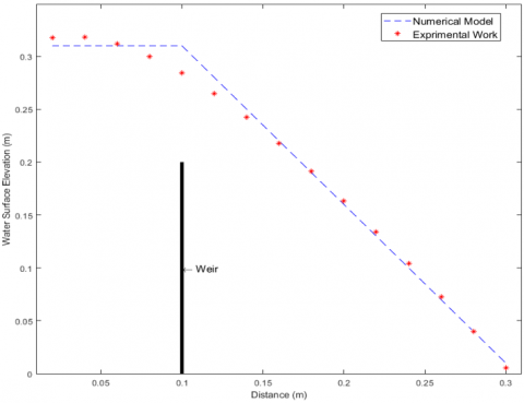
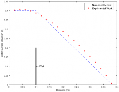
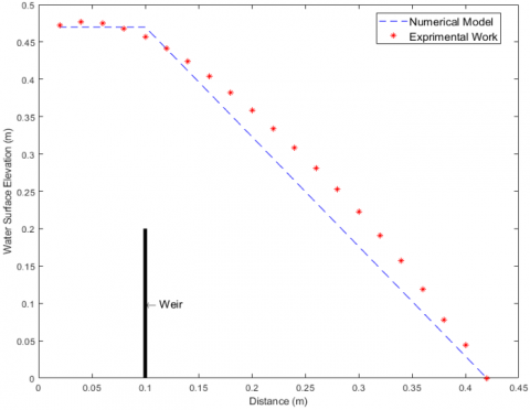
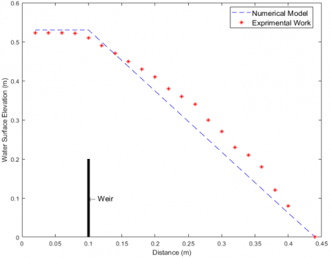
The explicit numerical solution was established according to the four-point box partial differential outline principle. The steady flow hydrograph was employed as an upstream boundary condition, while the known water depth (stage hydrograph) was used as a downstream boundary condition. Thus, the water surface elevation value would be estimated as a result of the numerical solution of Eqns. (11) and (12) simultaneously. Figures 4-10 show the correlation between the simulated water surface profile and the observed profile during the set of discharges previously mentioned in Table 1.

The results of comparing the calculated practically water surface levels with those calculated by the proposed numerical method, presented in the previous Figures 4-10, showed a great convergence. However, in order to evaluate the performance of the relationship between the amount of observed water surface elevation over the weir and the calculated values by the explicit numerical solution, a Nash-Sutcliff Error measurement was carried out based on the credibility and reliability of this methodology [22-24]. Eq. (13) represents the Nash-Sutcliff Error, where  is the measured quantity,  is the mimic quantity, and  is the mean of the measured quantity.

$N S E=1-\frac{\sum\left(h_{o b s}-h_{s i m} \;\;\; \right)^2}{\sum\left(h_{o b s}-\overline{h_{o b s}} \;\;\;\right)^2}$     (13)

The range of the Nash–Sutcliffe error is from 1 to −∞. If NSE=1, that means a great match of the mimicked to the measured variable. When the NSE=0, model forecasts are accurate to the average filed data. Finally, if the NSE < 0 indicates that the model simulation results are far from the average observed data.

Table 1 lists the value of NSE corresponding to each tested discharge in this study. It is noted that the average value of NSE=0.975 which is close to 1, indicating the high convergence between the values of the water level above the weir measured using the proposed explicit numerical model compared to the results obtained experimentally.

By observing the discharge of the water released, shown in Figures 4-10, over the weir used in this study, one can note that with the increase in the discharge values, there is a high agreement between the results obtained practically with those calculated theoretically. This is because an increase in the discharge will lead to an increase in the velocity head above the weir and, thus, an increase in the momentum force, making the water's surface push farther. On the other hand, as for the low discharges, it works to reduce the velocity head, which leads to a decrease in the momentum of the water and makes the curve of the water surface closer to the weir.

Table 1. The Nash–Sutcliffe error of the proposed approach

4.png

Figure 4. The shape of water surface profile flow=10 L/s

5.png

Figure 5. The shape of water surface profile flow=20 L/s

6.png

Figure 6. The shape of water surface profile flow=30 L/s

7.png

Figure 7. The shape of water surface profile flow=40 L/s

8.png

Figure 8. The shape of water surface profile flow=50 L/s

9.png

Figure 9. The shape of water surface profile flow=60 L/s

10.png

Figure 10. The shape of water surface profile flow=70 L/s