Yasir Ahmed Abdulameer*![]() | Abdulsattar Jaber Ali Al-Saif
| Abdulsattar Jaber Ali Al-Saif![]()
© 2023 IIETA. This article is published by IIETA and is licensed under the CC BY 4.0 license (http://creativecommons.org/licenses/by/4.0/).
OPEN ACCESS
In this study, a hybrid method combining the homotopy perturbation method (HPM) and Fourier transform (FT) is developed and denoted as FT-HPM. This novel algorithm leverages the properties of convolution theory to facilitate calculations and is applied to obtain approximate analytical solutions for the two-dimensional natural convection between two concentric horizontal circular cylinders maintained at various uniform temperatures. The effects of Rayleigh number, Prandtl number, and radius variation on the fluid flow (air) and heat transfer are investigated. Furthermore, velocity distributions are examined and discussed, while the Nusselt number is calculated to represent local and general heat transfer rates through the relevant Nusselt numbers. The convergence of the FT-HPM method is discussed theoretically, with the formulation of theorems that are applied to the results of the obtained solutions. Tables and graphs of the analytical solutions demonstrate the feasibility and potential usefulness of the proposed algorithm for addressing various nonlinear problems, particularly natural convection problems. This research contributes to the understanding of natural convection in complex geometries and provides a foundation for future studies in this field.
fourier transform, homotopy perturbation method, convolution theory, natural convection, cylindrical annuli
In recent years, the study of heat transfer theory due to natural convection has garnered significant interest among scientists and engineers, owing to its crucial applications in various scientific and technological fields. These applications encompass heat storage systems, cooling of electronic components, solar collectors, nuclear reactors, and aircraft cabin insulation, among others [1-3]. One particularly important problem in natural convection, which has intrigued numerous researchers, involves the phenomenon between two concentric horizontal circular cylinders maintained at varying uniform temperatures.
Early contributions to this area include the experimental solutions provided by Crawford and Lemlich [4], who conducted a numerical study to approximate the steady-state differential equations with suitable difference equations. Their work explored the effect of diameter ratios at 2, 8, and 57, in the case of a Prandtl number of 0.7. Subsequent researchers have built upon this foundation, developing numerical and analytical solutions to the problem. For instance, Mack and Bishop [5] performed an analytical investigation of natural convection between two horizontal circular concentric cylinders with small temperature differences. Their approach utilized Rayleigh number power series to solve the governing mathematical equations, and they discussed the characteristics of their solutions, such as local and global heat transfer rates, streamline formation, velocity, and temperature distributions. Additionally, they analyzed the effects of radius ratio, Prandtl number, and Rayleigh number.
Kuehn and Goldstein [1] employed the finite difference method in a numerical study to obtain experimental solutions for natural convection between two horizontal circular concentric cylinders. Tsui and Tremblay [6] conducted a theoretical-numerical study for Grashof numbers ranging from 7×10² to 9×10⁴, with a fixed Prandtl number of 0.7, and diameter ratio differences of 1.2, 1.5, and 2. Pop et al. [7] derived analytical solutions for transient natural convection between two concentric horizontal circular porous cylinders using the method of matched asymptotic expansions. Their approach divided the problem into three regions (inner boundary layer, core region, and outer boundary layer) and determined the analytical solutions for each region separately. They observed that their solutions markedly differed from steady-state solutions.
Sano and Kuribayashi [8] studied transient natural convection around a horizontal circular cylinder using the method of matched asymptotic expansions, resulting in new analytical solutions. Their research aimed to fill a gap in previous work by considering the displacement effect. Hassan and Al-Lateef [9] presented a numerical study to find the solution for two-dimensional transient natural convection heat transfer from isothermal horizontal cylindrical annuli. They employed the alternating direction implicit (ADI) method to solve both the vorticity and energy equations, while the stream function equation was solved using the successive over relaxation (SOR) method. Their results were summarized by Nussult number versus Grashof number curves, with diameter ratios and Prandtl number as parameters. Touzani et al. [10] numerically investigated natural convection in horizontal annulus with two heating blocks, noting that heat transfer was more significant in the upper region of the annulus and that the presence of the block improved overall heat transfer. Al-Saif and Al-Griffi [11] proposed a new algorithm that combined the homotopy perturbation method and the Yang transform to conduct an analytical study on the problem of two-dimensional transient natural convection between two concentric horizontal cylindrical annuli. Their work explored the effects of Grashof and Prandtl numbers, as well as the radius ratio, on heat transfer and fluid flow (air) at various values.
Despite the merits of the aforementioned methods and their capacity to find numerical and analytical solutions for non-linear problems, particularly in the context of heat transfer by natural convection, several challenges persist. These include high computational operations, time-consuming procedures, and the difficulty of using integral transformations (such as Laplace transform, Fourier transform, and Yang transform) to solve non-linear problems. To address these limitations, this study proposes a new algorithm combining the homotopy perturbation method (HPM) with the Fourier transform (FT), supported by the convolution theory, to create a hybrid procedure denoted as FT-HPM. This method leverages the convolution theory to reduce computational complexity related to integrative operations when using the homotopy perturbation method alone while also mitigating the difficulty of employing the Fourier transform to solve non-linear differential equations. The newly developed FT-HPM algorithm is applied to obtain approximate analytical solutions for the two-dimensional natural convection between two horizontal concentric cylinders. Tabular and graphical results of the new analytical approximate solutions demonstrate the usefulness, importance, and necessity of using this method. The accuracy and efficiency of this approach are validated by its agreement with the results of previous methods [10, 12, 13]. Furthermore, the convergence analysis of the solutions is studied both theoretically and experimentally by proving two theorems and deducing the necessary condition for the convergence of the method. The study also investigates the effect of Grashof number, Prandtl number, and radius ratio on the heat transfer and fluid flow in the annular space.
In 1988, He [14, 15] created the homotopy perturbation method (HPM). This method is considered highly effective and efficient in its ability to find solutions for linear and non-linear differential and integral equations. This method is characterized by its ability to solve many non-linear problems that have wide applications in various sciences and engineering. In this method, the solution can be considered as a summation of a convergent infinite series [16]. To provide a completed explanation of the idea of this method, we have to consider the general form of a non-linear differential equation:
$A(u)-q(r)=0, r \in \Omega$ (1)
subject to the following boundary conditions,
$B\left(u, \frac{\partial u}{\partial n}\right)=0, r \in \Gamma$ (2)
where, A refers to a general differential operator, u represents the unknown function, q(r) is a known analytic function, B denotes to the boundary operator, and Γ is the boundary of the domain Ω. The operator A can be divided into two operators, L and N, where L and N are a linear and non-linear operator, respectively. Moreover, Eq. (1) can be reformulated as follows:
$L(u)+N(u)-q(r)=0$ (3)
By the idea of the homotopy perturbation method, we assume a homotopy $U(r, p): \Omega \times[0,1] \rightarrow \mathbb{R}$ , which satisfies the following formula:
$\begin{gathered}H(U, p)=(1-p)\left[L(U)-L\left(u_0\right)\right]+p[A(U)-q(r)]=0\end{gathered}$ (4)
Or
$\begin{gathered}H(U, p)=L(U)-L\left(u_0\right)+p L\left(u_0\right)+p[N(U)-q(r)]=0\end{gathered}$ (5)
where, $p \in[0,1]$ denotes the impeding parameter and u0 is an initial condition for the solution of Eq. (1), which satisfies the boundary conditions. Clearly, from Eq. (4) or Eq. (5), we will get:
$\begin{gathered}H(U, 0)=L(U)-L\left(u_0\right)=0, \\ H(U, 1)=A(U)-q(r)=0.\end{gathered}$ (6)
Therefore, the solution of Eq. (4) or Eq. (5) can be expressed as a power series in terms of p by the following:
$U=\sum_{j=0}^{\infty} p^j U_j$ (7)
Putting p=1, then the approximate solution of Eq. (1) can be expressed as follow:
$u=\lim _{p \rightarrow 1} U=\sum_{j=0}^{\infty} U_j$ (8)
The main idea in this part is to improve the homotopy perturbation method by using the Fourier transform to get a new, more advanced procedure. To introduce the basic algorithm for this procedure, we rewrite Eq. (1) to get the following formula:
$L(U)+R(U)+N(U)=q(r)$ (9)
where, $L=\partial^n / \partial r^n$ represents to the linear differential operator, R and N refer to the linear differential operator such that its order is less than L, the general non-linear differential operator, respectively, and q(r) denotes the source term. Moreover, the main steps of this method can be stated as follows:
By using the HPM, we have:
$(1-p)\left[L(U)-L\left(u_0\right)\right]+p[A(U)-q(r)]=0$ (10)
Postulate that A(U)=L(U)+R(U)+N(U) and $L=\frac{\partial^n}{\partial r^n}$ , then, we deduce:
$\frac{\partial^n}{\partial r^n}(U)=\frac{\partial^n u_0}{\partial r^n}-p \frac{\partial^n u_0}{\partial r^n}-p[R(U)+N(U)-q(r)]$ (11)
By the effect of the Fourier transform on both sides of the Eq. (11), we get:
$\mathcal{F}\left[\frac{\partial^n}{\partial r^n}(U)\right]=\mathcal{F}\left[\frac{\partial^n u_0}{\partial r^n}\right]-p \mathcal{F}\left[\begin{array}{c}\frac{\partial^n}{\partial r^n}\left(u_0\right)+ \\ {[R(U)+N(U)-q(r)]}\end{array}\right]$ (12)
where, $\mathcal{F}[g(t)]=\mathcal{F}(\omega)=\int_{-\infty}^{\infty} g(t) e^{-i \omega t} d t$.
Using the differentiation property of the Fourier transform, we obtain:
$(i \omega)^n \mathcal{F}[U]=\mathcal{F}\left[\frac{\partial^n u_0}{\partial r^n}-p\left(\begin{array}{c}\frac{\partial^n}{\partial r^n}\left(u_0\right)+ \\ {[R(U)+N(U)-q(r)]}\end{array}\right)\right]$ (13)
The rearrangement of Eq. (13) leads to:
$\mathcal{F}[U]=\frac{1}{(i \omega)^n} \mathcal{F}\left[\frac{\partial^n u_0}{\partial r^n}-p\left(\begin{array}{c}\frac{\partial^n}{\partial r^n}\left(u_0\right)+ \\ {[R(U)+N(U)-q(r)]}\end{array}\right)\right]$ (14)
according to the properties of the Fourier transform, we get:
$\mathcal{F}[U]=\left\{\begin{array}{c}\frac{1}{2(n-1) !} \mathcal{F}\left[r^{n-1} \operatorname{sgn}(r)\right] \times \\ \mathcal{F}\left[\begin{array}{c}\frac{\partial^n}{\partial r^n}\left(u_0\right)- \\ p\left(\frac{\partial^n}{\partial r^n}\left(u_0\right)+[R(U)+N(U)-q(r)]\right)\end{array}\right]\end{array}\right\}$ (15)
where, $\mathcal{F}\left(t^n \operatorname{sgn}(t)\right)=(-i)^{n+1} \frac{2(n !)}{\omega^{n+1}}$ .
Applying the idea of convolution theory on the right-hand side of the Eq. (15) to get the following result:
$\mathcal{F}[U]=\mathcal{F}\left\{\left[\begin{array}{c}\frac{1}{2(n-1) !}\left[r^{n-1} \operatorname{sgn}(r)\right] * \\ \frac{\partial^n}{\partial r^n}\left(u_0\right)- \\ p\left(\frac{\partial^n}{\partial r^n}\left(u_0\right)+[R(U)+N(U)-q(r)]\right)\end{array}\right]\right\}$ (16)
where, the operation * is given by:
$\begin{gathered}f(t) * g(t)=\int_{-\infty}^{\infty} f(t-\eta) g(\eta) d \eta \equiv \int_{-\infty}^{\infty} f(\eta) g(t-\eta) d \eta \\ \text { and } \mathcal{F}[f(t) * g(t)]=\mathcal{F}[f(t)] * \mathcal{F}[g(t)].\end{gathered}$
By Taking the inverse Fourier transform for both sides of Eq. (16), we obtain:
$U=\left\{\frac{1}{2(n-1) !}\left[r^{n-1} \operatorname{sgn}(r)\right] *\left[\frac{\partial^n}{\partial r^n}\left(u_0\right)-p\left(\frac{\partial^n}{\partial r^n}\left(u_0\right)+[R(U)+N(U)-q(r)]\right)\right]\right\}$ (17)
Eq. (17) can be described as follows:
$U=\int_{-\infty}^{\infty}\left\{\begin{array}{c}{\left[\frac{(r-\eta)^{n-1} \operatorname{sgn}(r-\eta)}{2(n-1) !}\right] \times} \\ {\left.\left[\begin{array}{c}\frac{\partial^n}{\partial r^n}\left(u_0\right)-p \frac{\partial^n}{\partial r^n}\left(u_0\right)- \\ p\{R(U)+N(U)-q(r)\}\end{array}\right]\right|_{r=n}}\end{array}\right\} d \eta$ (18)
From the assumption of the HPM, we have:
$U=\sum_{m=0}^{\infty} p^j U_j$ (19)
and the non-linear terms can be decomposed as:
$N(U)=\sum_{j=0}^{\infty} p^j H_j$ (20)
where, Hj(U) represents the He’s polynomials [3] that are given by:
$\begin{gathered}H_j\left(U_0, U_1, U_2, \ldots, U_j\right)=\frac{1}{j !} \frac{\partial^j}{\partial p^j}\left[N\left(\sum_{i=0}^{\infty} p^i U_i\right)\right]_{p=0} \\ j=0,1,2,3, \ldots\end{gathered}$ (21)
Putting Eqns. (19) and (20) in to Eq. (18), we obtain:
$\sum_{m=0}^{\infty} p^j U_j=\int_{-\infty}^{\infty}\left\{\begin{array}{c}{\left[\frac{(r-\eta)^{n-1} \operatorname{sgn}(r-\eta)}{2(n-1) !}\right] \times} \\ {\left.\left[\frac{\partial^n u_0}{\partial r^n}-p\left(\frac{\partial^n u_0}{\partial r^n}+\left[\begin{array}{c}\left.R\left(\sum_{m=0}^{\infty} p^j U_j\right)+\right] \\ \sum_{j=0}^{\infty} p^j H_j-q(r)\end{array}\right]\right)\right]\right|_{r=\eta}}\end{array}\right\} d \eta$ (22)
By equating the coefficients of the same powers of p, we deduce:
$p^0: U_0=\int_{-\infty}^{\infty}\left\{\left.\left[\frac{(r-\eta)^{n-1} \operatorname{sgn}(r-\eta)}{2(n-1) !}\right]\left[\frac{\partial^n u_0}{\partial r^n}\right]\right|_{r=\eta}\right\} d \eta$ (23)
$p^1: U_1=-\int_{-\infty}^{\infty}\left\{\begin{array}{c}{\left[\frac{(r-\eta)^{n-1} \operatorname{sgn}(r-\eta)}{2(n-1) !}\right] \times} \\ {\left.\left[\frac{\partial^n u_0}{\partial r^n}+R\left(U_0\right)+H_0-q(r)\right]\right|_{r=\eta}}\end{array}\right\} d \eta$ (24)
$p^2: U_2=-\int_{-\infty}^{\infty}\left\{\begin{array}{c}{\left[\frac{(r-\eta)^{n-1} \operatorname{sgn}(r-\eta)}{2(n-1) !}\right] \times} \\ {\left.\left[R\left(U_1\right)+H_1\right]\right|_{r=\eta}}\end{array}\right\} d \eta$ (25)
$p^j: U_j=-\int_{-\infty}^{\infty}\left\{\begin{array}{c}{\left[\frac{(r-\eta)^{n-1} \operatorname{sgn}(r-\eta)}{2(n-1) !}\right] \times} \\ {\left.\left[R\left(U_{j-1}\right)+H_{j-1}\right]\right|_{r=\eta}}\end{array}\right\} d \eta$ (26)
Taking p=1, then the analytical approximate solution u can be given by:
$u=\lim _{p \rightarrow 1} U=\sum_{j=0}^{\infty} U_j$ (27)
Consider the two-dimensional steady laminar natural convection of a fluid bounded between two concentric horizontal circular cylinders. Let $\hat{r}_i$ refers to the radius of the inner cylinder, $\hat{r}_o=\hat{r}_i R$ the radius of the outer cylinder and $\hat{r}=\hat{r}_i r$ the radial coordinate (where $R$ denotes the radius ratio of the outer cylinder to that of the inner cylinder). Both cylinders are taken care at a various uniform temperature $\widehat{T}_i$ and $\widehat{T}_o$, respectively. In this case, it is assumed that gravity acts vertically downwards. In this study, cylindrical coordinates have been used, the coordinate angular $\theta$ measured counterclockwise from the downward vertical, $\theta=0$. Flow and temperature fields are assumed to be symmetric with respect to the vertical plane through the axis of the cylinders. The geometry diagram of the flow can be shown in Figure 1.
Figure 1. Cylindrical flow geometry and coordinate system
Now, the non-dimensional governing equations can be written [5] as:
$\begin{gathered}\nabla^4 \psi=\frac{1}{\operatorname{Pr}} \frac{1}{r}\left(\frac{\partial \psi}{\partial \theta} \frac{\partial \nabla^2 \psi}{\partial r}-\frac{\partial \psi}{\partial r} \frac{\partial \nabla^2 \psi}{\partial \theta}\right)+R a\left(\frac{\cos \theta}{r} \frac{\partial T}{\partial \theta}+\right. \left.\sin \theta \frac{\partial T}{\partial r}\right)\end{gathered}$ (28)
$\nabla^2 T=\frac{1}{r}\left(\frac{\partial \psi}{\partial \theta} \frac{\partial T}{\partial r}-\frac{\partial \psi}{\partial r} \frac{\partial T}{\partial \theta}\right)$ (29)
where, $R a=\hat{g} \hat{\beta}\left(\hat{T}_i-\hat{T}_O\right) \hat{r}_i^3 /(\hat{v} \hat{\alpha})$ denotes the Rayleigh number and $\operatorname{Pr}=\hat{v} / \hat{\alpha}$ denotes the Prandtl number, and the coefficients, $\hat{g}, \hat{\beta}, \hat{v}$ and $\hat{\alpha}$ refer to the acceleration of gravity, volumetric coefficient of thermal expansion, kinematic viscosity, and thermal diffusivity, respectively. And the operators $\nabla^4$ and $\nabla^2$ are defined by $\nabla^4=\nabla^2\left(\nabla^2\right)$ and $\nabla^2=$ $\frac{\partial^2}{\partial r^2}+\frac{1}{r} \frac{\partial}{\partial r}+\frac{1}{r^2} \frac{\partial^2}{\partial \theta^2}$.
The boundary conditions for Eqns. (28) and (29) in dimensionless form are given by:
$\left.\begin{array}{c}\psi=\frac{\partial \psi}{\partial r}=0, T=1 \text { at } r=1 \\ \psi=\frac{\partial \psi}{\partial r}=0, T=0 \text { at } r=R \\ \psi=\frac{\partial^2 \psi}{\partial \theta^2}=0, T=\frac{\partial T}{\partial \theta}=0 \text { at } \theta=0, \pi\end{array}\right\}$ (30)
Now, to apply the algorithm of FT-HPM, first, we simplify Eqns. (28) and (29) to get the following system:
$\begin{aligned} & \frac{\partial^4 \psi}{\partial r^4}+\frac{1}{r} \frac{\partial^3 \psi}{\partial r^3}+\frac{1}{r^2} \frac{\partial^4 \psi}{\partial \theta^2 \partial r^2}-\frac{1}{P r} \frac{1}{r}\left(\frac{\partial \psi}{\partial \theta} \frac{\partial \nabla^2 \psi}{\partial r}-\frac{\partial \psi}{\partial r} \frac{\partial \nabla^2 \psi}{\partial \theta}\right) \\ & +\nabla^2\left(\frac{1}{r} \frac{\partial \psi}{\partial r}+\frac{1}{r^2} \frac{\partial^2 \psi}{\partial \theta^2}\right)-R a\left(\frac{\cos \theta}{r} \frac{\partial T}{\partial \theta}+\sin \theta \frac{\partial T}{\partial r}\right)=0\end{aligned}$ (31)
$\frac{\partial^2 T}{\partial r^2}+\frac{1}{r} \frac{\partial T}{\partial r}+\frac{1}{r^2} \frac{\partial^2 T}{\partial \theta^2}-\frac{1}{r}\left(\frac{\partial \psi}{\partial \theta} \frac{\partial T}{\partial r}-\frac{\partial \psi}{\partial r} \frac{\partial T}{\partial \theta}\right)=0$ (32)
Then, the basic steps of the new technique for Eq. (31) and Eq. (32) are illustrated as follows.
By using HPM of Eq. (31) and Eq. (32), we obtain:
$\begin{aligned} & (1-p)\left[\frac{\partial^4 \psi}{\partial r^4}-\frac{\partial^4 \psi_0^*}{\partial r}\right]+ \\ & p\left[\begin{array}{l}\frac{\partial^4 \psi}{\partial r^4}+\frac{1}{r} \frac{\partial^3 \psi}{\partial r^3}+\frac{1}{r^2} \frac{\partial^4 \psi}{\partial \theta^2 \partial r^2}+\nabla^2\left(\frac{1}{r} \frac{\partial \psi}{\partial r}+\frac{1}{r^2} \frac{\partial^2 \psi}{\partial \theta^2}\right)- \\ \frac{1}{P r} \frac{1}{r}\left(\frac{\partial \psi}{\partial \theta} \frac{\partial \nabla^2 \psi}{\partial r}-\frac{\partial \psi}{\partial r} \frac{\partial \nabla^2 \psi}{\partial \theta}\right)-R a\left(\frac{\cos \theta}{r} \frac{\partial T}{\partial \theta}+\sin \theta \frac{\partial T}{\partial r}\right)\end{array}\right]=0 \\ & (1-p)\left[\frac{\partial^2 T}{\partial r^2}-\frac{\partial^2 T_0^*}{\partial r^2}\right]+p\left[\begin{array}{l}\frac{\partial^2 T}{\partial r^2}+\frac{1}{r} \frac{\partial T}{\partial r}+\frac{1}{r^2} \frac{\partial^2 T}{\partial \theta^2} \\ -\frac{1}{r}\left(\frac{\partial \psi}{\partial \theta} \frac{\partial T}{\partial r}-\frac{\partial \psi}{\partial r} \frac{\partial T}{\partial \theta}\right)\end{array}\right]=0 \\ & \end{aligned}$
where, $\psi_0^*$ and $T_0^*$ are the initial conditions. The rearrangement of the above equations yields:
$\frac{\partial^4 \psi}{\partial r^4}-\frac{\partial^4 \psi_0^*}{\partial r}+p \frac{\partial^4 \psi_0^*}{\partial r}+p\left[\begin{array}{c}\frac{1}{r} \frac{\partial^3 \psi}{\partial r^3}+\frac{1}{r^2} \frac{\partial^4 \psi}{\partial \theta^2 \partial r^2}-\frac{1}{P r} \frac{1}{r}\left(\frac{\partial \psi}{\partial \theta} \frac{\partial \nabla^2 \psi}{\partial r}-\frac{\partial \psi}{\partial r} \frac{\partial \nabla^2 \psi}{\partial \theta}\right)+ \\ \nabla^2\left(\frac{1}{r} \frac{\partial \psi}{\partial r}+\frac{1}{r^2} \frac{\partial^2 \psi}{\partial \theta^2}\right)-R a\left(\frac{\cos \theta}{r} \frac{\partial T}{\partial \theta}+\sin \theta \frac{\partial T}{\partial r}\right)\end{array}\right]=0$ (33)
$\begin{gathered}\frac{\partial^2 T}{\partial r^2}-\frac{\partial^2 T_0^*}{\partial r^2}+p\left[\frac{\partial^2 T_0^*}{\partial r^2}+\frac{1}{r} \frac{\partial T}{\partial r}+\frac{1}{r^2} \frac{\partial^2 T}{\partial \theta^2}-\frac{1}{r}\left(\frac{\partial \psi}{\partial \theta} \frac{\partial T}{\partial r}-\right.\right. \left.\left.\frac{\partial \psi}{\partial r} \frac{\partial T}{\partial \theta}\right)\right]=0\end{gathered}$ (34)
From the boundary conditions, the second and third terms in Eqns. (33) and (34) are equal to zero, therefore,
$\begin{aligned} & \frac{\partial^4 \psi}{\partial r^4}= \\ & -p\left[\begin{array}{c}\frac{1}{r} \frac{\partial^3 \psi}{\partial r^3}+\frac{1}{r^2} \frac{\partial^4 \psi}{\partial \theta^2 \partial r^2}-\frac{1}{\operatorname{Pr}} \frac{1}{r}\left(\frac{\partial \psi}{\partial \theta} \frac{\partial \nabla^2 \psi}{\partial r}-\frac{\partial \psi}{\partial r} \frac{\partial \nabla^2 \psi}{\partial \theta}\right)+ \\ \nabla^2\left(\frac{1}{r} \frac{\partial \psi}{\partial r}+\frac{1}{r^2} \frac{\partial^2 \psi}{\partial \theta^2}\right)-R a\left(\frac{\cos \theta}{r} \frac{\partial T}{\partial \theta}+\sin \theta \frac{\partial T}{\partial r}\right)\end{array}\right] \\ & \end{aligned}$ (35)
$\frac{\partial^2 T}{\partial r^2}=-p\left[\frac{1}{r} \frac{\partial T}{\partial r}+\frac{1}{r^2} \frac{\partial^2 T}{\partial \theta^2}-\frac{1}{r}\left(\frac{\partial \psi}{\partial \theta} \frac{\partial T}{\partial r}-\frac{\partial \psi}{\partial r} \frac{\partial T}{\partial \theta}\right)\right]$ (36)
Applying the Fourier transform with respect to r on both sides of Eq. (35) and Eq. (36), we have:
$\begin{gathered}\mathcal{F}\left[\frac{\partial^4 \psi}{\partial r^4}\right]= \\ -p \mathcal{F}\left[\begin{array}{c}\frac{1}{r} \frac{\partial^3 \psi}{\partial r^3}+\frac{1}{r^2} \frac{\partial^4 \psi}{\partial \theta^2 \partial r^2}-\frac{1}{P r} \frac{1}{r}\left(\frac{\partial \psi}{\partial \theta} \frac{\partial \nabla^2 \psi}{\partial r}-\frac{\partial \psi}{\partial r} \frac{\partial \nabla^2 \psi}{\partial \theta}\right)+ \\ \nabla^2\left(\frac{1}{r} \frac{\partial \psi}{\partial r}+\frac{1}{r^2} \frac{\partial^2 \psi}{\partial \theta^2}\right)-R a\left(\frac{\cos \theta}{r} \frac{\partial T}{\partial \theta}+\sin \theta \frac{\partial T}{\partial r}\right)\end{array}\right]\end{gathered}$ (37)
$\mathcal{F}\left[\frac{\partial^2 T}{\partial r^2}\right]=-p \mathcal{F}\left[\frac{1}{r} \frac{\partial T}{\partial r}+\frac{1}{r^2} \frac{\partial^2 T}{\partial \theta^2}-\frac{1}{r}\left(\frac{\partial \psi}{\partial \theta} \frac{\partial T}{\partial r}-\frac{\partial \psi}{\partial r} \frac{\partial T}{\partial \theta}\right)\right]$ (38)
Using the differentiation property of the Fourier transform, we deduce:
$(i \omega)^4 \mathcal{F}[\psi]=-p \mathcal{F}\left[\begin{array}{c}\frac{1}{r} \frac{\partial^3 \psi}{\partial r^3}+\frac{1}{r^2} \frac{\partial^4 \psi}{\partial \theta^2 \partial r^2}-\frac{1}{P r} \frac{1}{r}\left(\frac{\partial \psi}{\partial \theta} \frac{\partial \nabla^2 \psi}{\partial r}-\frac{\partial \psi}{\partial r} \frac{\partial \nabla^2 \psi}{\partial \theta}\right)+ \\ \nabla^2\left(\frac{1}{r} \frac{\partial \psi}{\partial r}+\frac{1}{r^2} \frac{\partial^2 \psi}{\partial \theta^2}\right)-R a\left(\frac{\cos \theta}{r} \frac{\partial T}{\partial \theta}+\sin \theta \frac{\partial T}{\partial r}\right)\end{array}\right]$ (39)
$(i \omega)^2 \mathcal{F}[T]=-p \mathcal{F}\left[\frac{1}{r} \frac{\partial T}{\partial r}+\frac{1}{r^2} \frac{\partial^2 T}{\partial \theta^2}-\frac{1}{r}\left(\frac{\partial \psi}{\partial \theta} \frac{\partial T}{\partial r}-\frac{\partial \psi}{\partial r} \frac{\partial T}{\partial \theta}\right)\right]$ (40)
The rearrangement of the above system leads to:
$\mathcal{F}[\psi]=\frac{1}{\omega^4} p \mathcal{F}\left[\begin{array}{c}\frac{1}{P r} \frac{1}{r}\left(\frac{\partial \psi}{\partial \theta} \frac{\partial \nabla^2 \psi}{\partial r}-\frac{\partial \psi}{\partial r} \frac{\partial \nabla^2 \psi}{\partial \theta}\right)-\frac{1}{r} \frac{\partial^3 \psi}{\partial r^3}-\frac{1}{r^2} \frac{\partial^4 \psi}{\partial \theta^2 \partial r^2}- \\ \nabla^2\left(\frac{1}{r} \frac{\partial \psi}{\partial r}+\frac{1}{r^2} \frac{\partial^2 \psi}{\partial \theta^2}\right)+R a\left(\frac{\cos \theta}{r} \frac{\partial T}{\partial \theta}+\sin \theta \frac{\partial T}{\partial r}\right)\end{array}\right]$ (41)
$\mathcal{F}[T]=\frac{1}{\omega^2} p \mathcal{F}\left[\frac{1}{r} \frac{\partial T}{\partial r}+\frac{1}{r^2} \frac{\partial^2 T}{\partial \theta^2}-\frac{1}{r}\left(\frac{\partial \psi}{\partial \theta} \frac{\partial T}{\partial r}-\frac{\partial \psi}{\partial r} \frac{\partial T}{\partial \theta}\right)\right]$ (42)
By using the properties of the Fourier transform, we get:
$\begin{gathered}\mathcal{F}[\psi]=p\left(\frac{1}{2(3 !)}\right) \mathcal{F}\left[r^3 \operatorname{sgn}(r)\right] \times \\ \mathcal{F}\left[\begin{array}{c}\frac{1}{\operatorname{Pr}} \frac{1}{r}\left(\frac{\partial \psi}{\partial \theta} \frac{\partial \nabla^2 \psi}{\partial r}-\frac{\partial \psi}{\partial r} \frac{\partial \nabla^2 \psi}{\partial \theta}\right)-\frac{1}{r} \frac{\partial^3 \psi}{\partial r^3}-\frac{1}{r^2} \frac{\partial^4 \psi}{\partial \theta^2 \partial r^2}- \\ \nabla^2\left(\frac{1}{r} \frac{\partial \psi}{\partial r}+\frac{1}{r^2} \frac{\partial^2 \psi}{\partial \theta^2}\right)+R a\left(\frac{\cos \theta}{r} \frac{\partial T}{\partial \theta}+\sin \theta \frac{\partial T}{\partial r}\right)\end{array}\right]\end{gathered}$ (43)
$\begin{gathered}\mathcal{F}[T]=p\left(\frac{-1}{2(1 !)}\right) \mathcal{F}[r \operatorname{sgn}(r)] \mathcal{F}\left[\frac{1}{r} \frac{\partial T}{\partial r}+\frac{1}{r^2} \frac{\partial^2 T}{\partial \theta^2}-\right. \\ \left.\frac{1}{r}\left(\frac{\partial \psi}{\partial \theta} \frac{\partial T}{\partial r}-\frac{\partial \psi}{\partial r} \frac{\partial T}{\partial \theta}\right)\right]\end{gathered}$ (44)
Applying the idea of convolution theory on the right-hand side of the above system to get the following result:
$\mathcal{F}[\psi]=\frac{p}{12} \mathcal{F}\left\{\left[\begin{array}{c}{\left[r^3 \operatorname{sgn}(r)\right] *} \\ \left.\frac{1}{P r} \frac{1}{r}\left(\frac{\partial \psi}{\partial \theta} \frac{\partial \nabla^2 \psi}{\partial r}-\frac{\partial \psi}{\partial r} \frac{\partial \nabla^2 \psi}{\partial \theta}\right)-\frac{1}{r} \frac{\partial^3 \psi}{\partial r^3}-\frac{1}{r^2} \frac{\partial^4 \psi}{\partial \theta^2 \partial r^2}-\right] \\ \nabla^2\left(\frac{1}{r} \frac{\partial \psi}{\partial r}+\frac{1}{r^2} \frac{\partial^2 \psi}{\partial \theta^2}\right)+R a\left(\frac{\cos \theta}{r} \frac{\partial T}{\partial \theta}+\sin \theta \frac{\partial T}{\partial r}\right)\end{array}\right]\right\}$ (45)
$\mathcal{F}[T]=\frac{p}{2} \mathcal{F}\left\{[r s g n(r)] *\left[\begin{array}{c}\frac{1}{r}\left(\frac{\partial \psi}{\partial \theta} \frac{\partial T}{\partial r}-\frac{\partial \psi}{\partial r} \frac{\partial T}{\partial \theta}\right) \\ -\frac{1}{r} \frac{\partial T}{\partial r}-\frac{1}{r^2} \frac{\partial^2 T}{\partial \theta^2}\end{array}\right]\right\}$ (46)
Taking the Fourier inverse for both sides of Eqns. (45) and (46) we get:
$\psi=\frac{1}{12} p\left\{\left[\begin{array}{c}{\left[r^3 \operatorname{sgn}(r)\right] *} \\ \frac{1}{P r} \frac{1}{r}\left(\frac{\partial \psi}{\partial \theta} \frac{\partial \nabla^2 \psi}{\partial r}-\frac{\partial \psi}{\partial r} \frac{\partial \nabla^2 \psi}{\partial \theta}\right)-\frac{1}{r} \frac{\partial^3 \psi}{\partial r^3}-\frac{1}{r^2} \frac{\partial^4 \psi}{\partial \theta^2 \partial r^2}- \\ \nabla^2\left(\frac{1}{r} \frac{\partial \psi}{\partial r}+\frac{1}{r^2} \frac{\partial^2 \psi}{\partial \theta^2}\right)+R a\left(\frac{\cos \theta}{r} \frac{\partial T}{\partial \theta}+\sin \theta \frac{\partial T}{\partial r}\right)\end{array}\right]\right\}$ (47)
$T=\frac{1}{2} p\left\{[r \operatorname{sgn}(r)] *\left[\begin{array}{c}\frac{1}{r}\left(\frac{\partial \psi}{\partial \theta} \frac{\partial T}{\partial r}-\frac{\partial \psi}{\partial r} \frac{\partial T}{\partial \theta}\right) \\ -\frac{1}{r} \frac{\partial T}{\partial r}-\frac{1}{r^2} \frac{\partial^2 T}{\partial \theta^2}\end{array}\right]\right\}$ (48)
Eq. (47) and Eq. (48) can be described as follows:
$\psi=\int_{-\infty}^{\infty}\left\{\left[\begin{array}{c}\frac{1}{12} p\left[(r-\eta)^3 \operatorname{sgn}(r-\eta)\right] \times \\ {\left.\left[\begin{array}{c}\frac{1}{P r} \frac{1}{r}\left(\frac{\partial \psi}{\partial \theta} \frac{\partial \nabla^2 \psi}{\partial r}-\frac{\partial \psi}{\partial r} \frac{\partial \nabla^2 \psi}{\partial \theta}\right)-\frac{1}{r} \frac{\partial^3 \psi}{\partial r^3}-\frac{1}{r^2} \frac{\partial^4 \psi}{\partial \theta^2 \partial r^2}- \\ \nabla^2\left(\frac{1}{r} \frac{\partial \psi}{\partial r}+\frac{1}{r^2} \frac{\partial^2 \psi}{\partial \theta^2}\right)+R a\left(\frac{\cos \theta}{r} \frac{\partial T}{\partial \theta}+\sin \theta \frac{\partial T}{\partial r}\right)\end{array}\right]\right|_{r=\eta}}\end{array}\right\} d \eta\right.$ (49)
$T=\frac{1}{2} p \int_{-\infty}^{\infty}\left\{\begin{array}{c}{[(r-\eta) \operatorname{sgn}(r-\eta)] \times} \\ {\left.\left[\frac{1}{r}\left(\frac{\partial \psi}{\partial \theta} \frac{\partial T}{\partial r}-\frac{\partial \psi}{\partial r} \frac{\partial T}{\partial \theta}\right)-\frac{1}{r} \frac{\partial T}{\partial r}-\frac{1}{r^2} \frac{\partial^2 T}{\partial \theta^2}\right]\right|_{r=\eta}}\end{array}\right\} d \eta$ (50)
From the assumption of the HPM, we have:
$\psi=\sum_{m=0}^{\infty} p^j \psi_j$ and $T=\sum_{m=0}^{\infty} p^j T_j$ (51)
and the nonlinear terms can be represented as:
$\left.\begin{array}{l}\frac{\partial \psi}{\partial \theta} \frac{\partial \nabla^2 \psi}{\partial r}=\sum_{j=0}^{\infty} p^j H_j, \frac{\partial \psi}{\partial r} \frac{\partial \nabla^2 \psi}{\partial \theta}=\sum_{j=0}^{\infty} p^j H_j^* \\ \frac{\partial \psi}{\partial \theta} \frac{\partial T}{\partial r}=\sum_{j=0}^{\infty} p^j G_j \text { and } \frac{\partial \psi}{\partial r} \frac{\partial T}{\partial \theta}=\sum_{j=0}^{\infty} p^j G_j^*\end{array}\right\}$ (52)
Substituting Eqns. (51) and (52) in Eqns. (49) and (50), we get:
$\begin{gathered}\sum_{j=0}^{\infty} p^j \psi_j=\int_{-\infty}^{\infty}\left\{p\left[\frac{(r-\eta)^3 \operatorname{sgn}(r-\eta)}{12}\right] \times\left[\frac{1}{P r} \frac{1}{r}\left(\sum_{j=0}^{\infty} p^j H_j-\sum_{j=0}^{\infty} p^j H_j^*\right)-\frac{1}{r^2} \frac{\partial^4}{\partial \theta^2 \partial r^2} \sum_{j=0}^{\infty} p^j \psi_j-\frac{1}{r} \frac{\partial^3}{\partial r^3} \sum_{j=0}^{\infty} p^j \psi_j-\nabla^2\left(\frac{1}{r} \frac{\partial}{\partial r} \sum_{j=0}^{\infty} p^j \psi_j+\right.\right.\right. \\ \left.\left.\left.\frac{1}{r^2} \frac{\partial^2}{\partial \theta^2} \sum_{j=0}^{\infty} p^j \psi_j\right)+R a\left(\frac{\cos \theta}{r} \frac{\partial}{\partial \theta} \sum_{j=0}^{\infty} p^j T_j+\sin \theta \frac{\partial}{\partial r} \sum_{j=0}^{\infty} p^j T_j\right)\right]\left.\right|_{r=\eta}\right\} d \eta\end{gathered}$ (53)
$\sum_{j=0}^{\infty} p^j T_j=\int_{-\infty}^{\infty}\left\{p\left[\frac{(r-\eta) \operatorname{sgn}(r-\eta)}{2}\right] \times\left.\left[\begin{array}{c}\frac{1}{r}\left(\sum_{j=0}^{\infty} p^j G_j-\sum_{j=0}^{\infty} p^j G_j^*\right)- \\ \frac{1}{r} \frac{\partial}{\partial r} \sum_{j=0}^{\infty} p^j T_j-\frac{1}{r^2} \frac{\partial^2}{\partial \theta^2} \sum_{j=0}^{\infty} p^j T_j\end{array}\right]\right|_{r=\eta}\right\} d \eta$ (54)
Comparing the coefficients of the same powers of p, we obtain:
$p^0:\left\{\begin{array}{c}\psi_0=\int_{-\infty}^{\infty}\left\{\left.\left[\frac{(r-\eta)^3 \operatorname{sgn}(r-\eta)}{12}\right][0]\right|_{r=\eta}\right\} d \eta \Rightarrow \\ (i \omega)^4 \mathcal{F}[\psi]=0 \Rightarrow \frac{\partial^4 \psi_0}{\partial r^4}=0 \\ T_0=\int_{-\infty}^{\infty}\left\{\left.\left[\frac{(r-\eta) \operatorname{sgn}(r-\eta)}{2}\right][0]\right|_{r=\eta}\right\} d \eta \Rightarrow \\ (i \omega)^2 \mathcal{F}[T]=0 \Rightarrow \frac{\partial^2 T_0}{\partial r^2}=0\end{array}\right.$ (55)
$p^1:\left\{\begin{array}{l}\psi_1=\int_{-\infty}^{\infty}\left\{\left[\frac{(r-\eta)^3 \operatorname{sgn}(r-\eta)}{12}\right] \times\left.\left[\frac{1}{P r} \frac{1}{r}\left(H_0-H_0^*\right)-\frac{1}{r^2} \frac{\partial^4 \psi_0}{\partial \theta^2 \partial r^2}+R a\left(\frac{\cos \theta}{r} \frac{\partial T_0}{\partial \theta}+\sin \theta \frac{\partial T_0}{\partial r}\right)-\frac{1}{r} \frac{\partial^3 \psi_0}{\partial r^3}-\nabla^2\left(\frac{1}{r} \frac{\partial \psi_0}{\partial r}+\frac{1}{r^2} \frac{\partial^2 \psi_0}{\partial \theta^2}\right)\right]\right|_{r=\eta}\right\} d \eta \\ T_1=\int_{-\infty}^{\infty}\left\{\left[\frac{(r-\eta) \operatorname{sgn}(r-\eta)}{2}\right] \times\left.\left[\frac{1}{r}\left(G_0-G_0^*\right)-\frac{1}{r} \frac{\partial T_0}{\partial r}-\frac{1}{r^2} \frac{\partial^2 T_0}{\partial \theta^2}\right]\right|_{r=\eta}\right\} d \eta\end{array}\right.$ (56)
$p^2:\left\{\begin{array}{c}\psi_2=\int_{-\infty}^{\infty}\left\{\left[\frac{(r-\eta)^3 \operatorname{sgn}(r-\eta)}{12}\right] \times\left.\left[\frac{1}{\operatorname{Pr}} \frac{1}{r}\left(H_1-H_1^*\right)-\frac{1}{r^2} \frac{\partial^4 \psi_1}{\partial \theta^2 \partial r^2}+R a\left(\frac{\cos \theta}{r} \frac{\partial T_1}{\partial \theta}+\sin \theta \frac{\partial T_1}{\partial r}\right)-\frac{1}{r} \frac{\partial^3 \psi_1}{\partial r^3}-\nabla^2\left(\frac{1}{r} \frac{\partial \psi_1}{\partial r}+\frac{1}{r^2} \frac{\partial^2 \psi_1}{\partial \theta^2}\right)\right]\right|_{r=\eta}\right\} d \eta \\ T_2=\int_{-\infty}^{\infty}\left\{\left[\frac{(r-\eta) \operatorname{sgn}(r-\eta)}{2}\right] \times\left.\left[\frac{1}{r}\left(G_1-G_1^*\right)-\frac{1}{r} \frac{\partial T_1}{\partial r}-\frac{1}{r^2} \frac{\partial^2 T_1}{\partial \theta^2}\right]\right|_{r=\eta}\right\} d \eta\end{array}\right.$ (57)
$p^j:\left\{\begin{array}{c}\psi_j=\int_{-\infty}^{\infty}\left\{\left[\frac{(r-\eta)^3 \operatorname{sgn}(r-\eta)}{12}\right] \times\left.\left[\frac{1}{P r} \frac{1}{r}\left(H_{j-1}-H_{j-1}^*\right)-\frac{1}{r^2} \frac{\partial^4 \psi_{j-1}}{\partial \theta^2 \partial r^2}+R a\left(\frac{\cos \theta}{r} \frac{\partial T_{j-1}}{\partial \theta}+\sin \theta \frac{\partial T_{j-1}}{\partial r}\right)-\frac{1}{r} \frac{\partial^3 \psi_{j-1}}{\partial r^3}-\nabla^2\left(\frac{1}{r} \frac{\partial \psi_{j-1}}{\partial r}+\frac{1}{r^2} \frac{\partial^2 \psi_{j-1}}{\partial \theta^2}\right)\right]\right|_{r=\eta}\right\} d \eta \\ T_j=\int_{-\infty}^{\infty}\left\{\left[\frac{(r-\eta) \operatorname{sgn}(r-\eta)}{2}\right] \times\left.\frac{1}{r}\left[\left(G_{j-1}-G_{j-1}^*\right)-\frac{\partial T_{j-1}}{\partial r}-\frac{1}{r} \frac{\partial^2 T_{j-1}}{\partial \theta^2}\right]\right|_{r=\eta}\right\} d \eta\end{array}\right.$ (58)
where,
$\left.\begin{array}{c}H_0=\frac{\partial \psi_0}{\partial \theta} \frac{\partial \nabla^2 \psi_0}{\partial r}, H_1=\frac{\partial \psi_0}{\partial \theta} \frac{\partial \nabla^2 \psi_1}{\partial r}+\frac{\partial \psi_1}{\partial \theta} \frac{\partial \nabla^2 \psi_0}{\partial r} \\ H_0^*=\frac{\partial \psi_0}{\partial r} \frac{\partial \nabla^2 \psi_0}{\partial \theta}, H_1^*=\frac{\partial \psi_0}{\partial r} \frac{\partial \nabla^2 \psi_1}{\partial \theta}+\frac{\partial \psi_1}{\partial r} \frac{\partial \nabla^2 \psi_0}{\partial \theta} \\ G_0=\frac{\partial \psi_0}{\partial \theta} \frac{\partial T_0}{\partial r}, G_1=\frac{\partial \psi_0}{\partial \theta} \frac{\partial T_1}{\partial r}+\frac{\partial \psi_1}{\partial \theta} \frac{\partial T_0}{\partial r} \\ G_0^*=\frac{\partial \psi_0}{\partial r} \frac{\partial T_0}{\partial \theta} \text { and } G_1^*=\frac{\partial \psi_0}{\partial r} \frac{\partial T_1}{\partial \theta}+\frac{\partial \psi_1}{\partial r} \frac{\partial T_0}{\partial \theta}\end{array}\right\}$ (59)
To solve Eq. (55), we use the integration with respect to r subject to the boundary conditions in Eq. (30), to get:
$\psi_0=\phi(\theta)\left(\begin{array}{c}\frac{1}{6} r^3-\frac{R+1}{4} r^2+\frac{R}{2} r+ \\ \frac{1}{24}\left(R^3-3 R^2-3 R+1\right)\end{array}\right), T_0=\frac{(R-r)}{R-1}$ (60)
$\psi_1=\frac{1}{48} \frac{1}{\left(R^2-R\right)}\left[\begin{array}{c}-R a R\left\{\begin{array}{c}2 r^4-4(R+1) r^3+6\left(R^2+1\right) r^2 \\ -4\left(R^3+1\right) r+R^4+1\end{array}\right\} \sin \theta \\ -\frac{1}{M}\left\{\begin{array}{c}2 R a R(R-1)\left(R^3-3 R^2+3 R-1\right) \\ \times\left[\left(-3 R r^3-3 R^2 r\right) \ln (R)+\ldots\right]\end{array}\right\} \sin \theta\end{array}\right]$ (61)
$T_1=\frac{1}{144} \frac{1}{(R-1)}\left[\begin{array}{c}\frac{3}{M} R a R(R-1)^3 \times \\ \left\{\begin{array}{c}r(R+1)\left(R^2-4 R+1\right)\left(\begin{array}{c}\ln (R)- \\ 2 \ln (r)\end{array}\right) \\ +\left(2 r^3-12 r^2+3 r-2\right) R-\frac{2}{3} r^4+ \\ 2 r^3+(2 r+6) R^2+6\left(R^2+1\right) r^2 \\ +\frac{1}{3} r-\left(\frac{1}{3} r-2\right) R^3\end{array}\right\} \cos (\theta) \\ -\frac{144}{2}((2 \ln (r)-\ln (R)-2) r+R+1)\end{array}\right]$ (62)
$\psi_2=\frac{1}{144} \frac{\operatorname{Raln}(R)}{(R-1) M}\left[\begin{array}{c}\left(72 r^4+390 r^3-54 r^2-9 r+6\right) R \\ +72 R \ln (R)(R+1)^2 r^3-15 r^3- \\ 36 R r^3\left(\begin{array}{l}-4 R^3+10 R^2 \\ +R^4+4 R+5\end{array}\right) \ln (r)+\cdots+ \\ \left(\begin{array}{c}-\frac{9671}{735}-\frac{24067}{210} r-\frac{1766}{7} r^2+\frac{26525}{42} r^3 \\ +\frac{2200}{3} r^4-\frac{9873}{35} r^5+\frac{3064}{35} r^6-\frac{2048}{147} r^7\end{array}\right) \\ \quad \times\left(\frac{7(R-1) \cos (\theta) R a}{160 P r \ln (R) M}\right) R^2+\cdots\end{array}\right] \sin \theta$ (63)
$T_2=\frac{31(R-1)^3 R a}{161280 M^2}$$\left[\begin{array}{c}\frac{140 R a}{31}\left(R^3-4 R^2+R\right)(R+1) r \times \\ \left(\begin{array}{c}\left(R^3-3 R^2+3 R+1\right) \ln (r) \ln (R) \\ +\cdots\end{array}\right) \\ +\left(\begin{array}{c}\frac{35}{31}-\frac{280}{31} r-\frac{560}{31} r^2-\frac{840}{31} r^3 \\ +\frac{2870}{31} r^4-\frac{1400}{31} r^5+\frac{560}{93} r^6\end{array}\right) R^2+\cdots\end{array}\right]$$\cos \theta$ (64)
where
$\begin{gathered}\phi(\theta)=\frac{\left(R^3-3\left(R^2-R\right)+1\right)}{M} \sin \theta, \\ M=\left[6\left(R^2+R\right) \ln (R)-2 R^4+7 R^3-21 R^2+17 R-1\right] .\end{gathered}$
The analytical approximate solutions ψ, T are given by putting p=1 as:
$\psi=\lim _{N \rightarrow \infty} \sum_{j=0}^N \psi_j$ (65)
$T=\lim _{N \rightarrow \infty} \sum_{j=0}^N T_j$ (66)
In this part, we will discuss the results of the new procedure (FT-HPM), which was used to solve the two-dimensional natural convection problem between two concentric horizontal. The dimensionless parameter Rayleigh number and the diameter ratio are used, which significantly influence the flow pattern, mechanism of the heat transfer and the stability of flow transfers in the system (28, 29).
6.1 Streamline and isotherm patterns
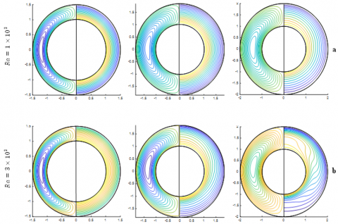
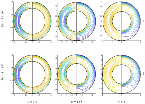
To illustrate the heat transfer within the cylinders, the streamlines and isotherm contours are used. In Figure 2-a, b, c, d, the Rayleigh number of the range (103≤Ra≤104) as well as different diameter ratios (R=1.5, 1.85 and 2.0) at Prandtl number of 0.7 are considered.
Figure 2-a shows that there is no significant change in the flow pattern and temperature fields at Ra=103 with different values of diameter ratio. The flow of fluid and temperature for Ra=3×10³, Pr=0.7, at different diameter ratios (R=1.5, 1.85 and 2.0) are illustrated in Figure 2-b. It is clear in this figure, that the flow pattern starts with the upward displacement, even if slightly, with the increase in the radius ratio. Moreover, the temperature pattern looks like circles when the radius is between R=1.5 and R=1.85, due to the weak effect of convection currents, while the temperature pattern appears distorted at R=2, this indicates that an increase in the heat convection. Figure 2-c explain the effect of Ra=5×10³, Pr=0.7, with different diameter ratios R. In this figure, we notice that the flow pattern moves upwards as the radius ratio increases. While the temperature pattern resembles circles when the radius ratio is R=1.5 and the effect of heat currents increases with increasing the diameter ratio to R=1.85 and when the radius ratio is increased to R=2, the temperature pattern becomes more distorted. It is clear from Figure 2-d that the increase in the Rayleigh number and the diameter ratio leads to a distortion of the temperature distribution. From the plot of streamlines and isotherms at Rayleigh number of 104, the radial temperature inversion appears indicating the separation of the inner and outer cylinder thermal boundary layers which is obvious at R=2.
Table 1. Comparison of absolute error between FT-HPM and HPM of ψ(r,θ) at Ra=1000 and Pr=0.7
|
θ |
R |
r=1.1 |
r=1.5 |
||
|
FT-HPM |
HPM |
FT-HPM |
HPM |
||
|
0 |
1.5 |
0.0000 |
0.0000 |
0.0000 |
0.0000 |
|
2 |
0.0000 |
0.0000 |
0.0000 |
0.0000 |
|
|
30 |
1.5 |
0.18×10⁻⁵ |
0.28×10⁻³ |
0.25×10⁻³ |
7.22×10⁻¹ |
|
2 |
0.20×10⁻⁵ |
0.77×10⁻³ |
0.38×10⁻³ |
3.61×10⁻¹ |
|
|
60 |
1.5 |
4.70×10⁻⁷ |
0.12×10⁻² |
0.13×10⁻³ |
3.64×10⁻¹ |
|
2 |
8.53×10⁻⁷ |
0.85×10⁻³ |
0.52×10⁻³ |
1.0084 |
|
|
90 |
1.5 |
0.15×10⁻⁵ |
0.21×10⁻² |
0.10×10⁻² |
2.83×10⁻¹ |
|
2 |
0.22×10⁻⁵ |
0.16×10⁻² |
0.99×10⁻³ |
1.45 |
|
|
180 |
1.5 |
0.13×10⁻⁵ |
0.23×10⁻² |
0.16×10⁻³ |
4.64×10⁻¹ |
|
2 |
0.20×10⁻⁵ |
0.17×10⁻² |
0.10×10⁻² |
1.7091 |
|
Table 2. Comparison of absolute error between FT-HPM and HPM of T(r,θ) at Ra=1000 and Pr=0.7
|
θ |
R |
r=1.1 |
r=1.5 |
||
|
FT-HPM |
HPM |
FT-HPM |
HPM |
||
|
0 |
1.5 |
0.13×10⁻⁴ |
0.66×10⁻² |
0.11×10⁻⁴ |
0.82×10⁻¹ |
|
2 |
0.95×10⁻³ |
0.12×10⁻¹ |
1.24×10⁻³ |
2.27×10⁻¹ |
|
|
30 |
1.5 |
0.88×10⁻⁵ |
0.19×10⁻² |
0.20×10⁻⁴ |
0.33×10⁻¹ |
|
2 |
0.14×10⁻² |
0.23×10⁻² |
0.93×10⁻³ |
0.45×10⁻¹ |
|
|
60 |
1.5 |
0.16×10⁻⁴ |
0.41×10⁻² |
0.12×10⁻⁵ |
0.31×10⁻¹ |
|
2 |
0.11×10⁻² |
0.10×10⁻¹ |
1.03×10⁻³ |
1.92×10⁻¹ |
|
|
90 |
1.5 |
0.11×10⁻⁴ |
0.14×10⁻² |
0.16×10⁻⁴ |
0.21×10⁻² |
|
2 |
0.14×10⁻² |
0.46×10⁻² |
0.53×10⁻³ |
0.84×10⁻¹ |
|
|
180 |
1.5 |
0.12×10⁻⁴ |
0.22×10⁻² |
0.12×10⁻⁴ |
0.10×10⁻¹ |
|
2 |
0.13×10⁻² |
0.64×10⁻² |
1.87×10⁻⁴ |
1.16×10⁻¹ |
|
In the above Tables 1 and 2, the absolute errors of the approximate solutions obtained using FT-HPM and HPM were compared at Ra=1000 and Pr=0.7. It is clear from these tables that the absolute errors using FT-HPM are lower than the absolute errors using HPM, moreover, we find that the new method (FT-HPM) has higher accuracy and efficiency than HPM.
Figure 2. Streamline (left) and isotherms (right) at different rayleigh number, Pr=0.7
6.2 Velocity distribution
In the $r$ - and $\theta$-directions, the components of velocity $\widehat{V}_r=$ $\hat{\alpha} \hat{r}_i^{-1} V_r(r, \theta)$ and $\hat{V}_\theta=\hat{\alpha} \hat{r}_i^{-1} V_\theta(r, \theta)$, can be calculated by using the following relations, respectively:
$V_r=\frac{1}{r} \frac{\partial \psi}{\partial \theta}, V_\theta=-\frac{\partial \psi}{\partial r}$ (67)
In Figure 3 we plot the velocity Vθ, obtained by differentiation of Eq. (65) with respect to r, for θ=n(30°), 1<n<5 at Ra=3000, Pr=0.7, and R=1.85.
Figure 3. $\theta$ -component of velocity versus radial position at θ=n(30°), 1<n<5 at Ra=3000, Pr=0.7, and R=1.85
As is evident from Figure 3, for the creeping-flow solution, Vθ(r,θ) and Vθ(r,π-θ) are equal, while, such symmetry does not hold for finite Rayleigh numbers. The velocity has a maximum value in the up-flow region occupying roughly that half of the gap which is nearer the inner cylinder, while the minimum velocity is in the down flow region in the outer ‘half’ gap. It was noted that the magnitude of maximum is in the following order, greatest for θ=90°, next greatest for 120°, followed by 60°, 150°, and 30°, While in minimum, the absolute magnitude is equally great for θ=90° and 120°. In addition, it is found that the magnitudes of the extrema in the upper half are larger than those corresponding in the lower half of the flow region. For θ=120°, both extremes are approximately equal. The maximum for the velocity Vθ has the largest magnitude for any θ between 0° and 120°, while the minimum has the largest magnitude when θ is between 120° and 180°.
6.3 Heat transfer rates
The local Nusselt numbers $N u_i(\theta)$ and $N u_o(\theta)$ are used to express the local heat flow rates per unit area as $\hat{q}_i=$ $\hat{k}\left(\widehat{T}_i-\widehat{T}_o\right) \hat{r}_i^{-1} \ln (R)^{-1} N u_i \quad$ and $\quad \hat{q}_o=\hat{k}\left(\widehat{T}_i-\right.$ $\left.\widehat{T}_O\right) \hat{r}_i^{-1} R^{-1} \ln (R)^{-1} N u_o$ in the inner and outer cylinders, respectively, where $\hat{k}$ denotes to the thermal conductivity of the fluid. In the same way, the means of the overall Nusselt number $\overline{N u}$ is used to express the total heat flow rate $\hat{Q}$ from the inner cylinder to the outer cylinder as $\hat{Q}=\pi \hat{k}\left(\hat{T}_i-\right.$ $\left.\widehat{T}_O\right) \ln (R)^{-1} \overline{N u}$. Moreover, by the Fourier's law of conduction, the local Nusselt numbers $N u_i(\theta)$ and $N u_o(\theta)$, and the mean Nusselt number $\overline{N u}$ are defined respectively as follows:
$N u_i=-\ln (R)\left[r \frac{\partial T}{\partial r}\right]_{r=1}$ (68)
$N u_o=-\ln (R)\left[r \frac{\partial T}{\partial r}\right]_{r=R}$ (69)
$\overline{N u}=-\frac{\ln (R)}{\pi} \int_0^\pi\left[r \frac{\partial T}{\partial r}\right]_{r=1} d \theta=-\frac{\ln (R)}{\pi} \int_0^\pi\left[r \frac{\partial T}{\partial r}\right]_{r=R} d \theta$ (70)
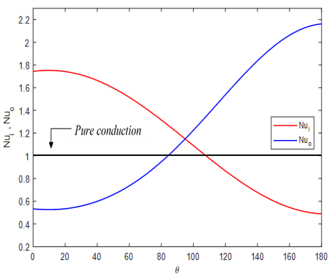
The effect of Ra=3000, Pr=0.7, and R=1.85 is appeared in Figure 4. In this figure, the local Nusselt numbers Nuiand Nuo are represented as functions of θ. It is observed from Figure 4 that Nui>1 at 0°<θ<110°, and that Nui<1 at 110°<θ<180°, whereas Nuo<1 at 0°<θ<85°, and Nuo>1 at 85°<θ<180°. That is mean, the rate of heat transfer has been increased in the lower and upper ‘half’ of the inner and outer cylinders, respectively, while the rate of heat transfer has been reduced in another region. Of the two maxima, the greatest value of Nuo occurring at θ=180°. Whereas, of the two minima, at θ=180° the Nusselt number Nui has absolute difference which is greater than unity (the pure conduction value of Nusselt number). It is clear that the mean ordinate for both curves in Figure 4 is greater than unity.
Figure 4. Inner cylinder and outer cylinder local nusselt numbers versus angular position for Ra=3000, Pr=0.7, and R=1.85
In Table 3, the maximum value of stream function $\psi_{\max }$ and the average Nusselt number $\overline{N u}$ between the present study and two methods, namely the ADI method and the SamarskiiAndreev method [12] are compared for Rayleigh numbers of $20,30,80,100$ and 200 and radius ratios of 2 and $\sqrt{2}$. In addition, Table 4 shows a comparison of the average Nusselt number for the present work with that of Singh et al. [13] and Zhang et al. [17] for Rayleigh numbers of $10^3$ and $10^4$.
Table 3. Comparison with ADI and samarskii-andreev methods [12] at Pr=0.7 with different values of rayleigh number
|
Ra |
R |
ψmax |
Nu |
||||
|
FT-HPM |
ADI |
Samarskii-Andreev |
FT-HPM |
ADI |
Samarskii-Andreev |
||
|
20 |
2 |
2.338 |
2.338 |
2.339 |
1.066 |
1.066 |
1.067 |
|
30 |
3.461 |
3.461 |
3.463 |
1.143 |
1.143 |
1.143 |
|
|
100 |
9.986 |
9.971 |
9.971 |
1.807 |
1.868 |
1.868 |
|
|
200 |
16.31 |
16.31 |
16.31 |
2.691 |
2.691 |
2.691 |
|
|
20 |
$2^{\frac{1}{2}}$ |
1.020 |
1.020 |
1.020 |
1.003 |
1.003 |
1.003 |
|
30 |
1.528 |
1.528 |
1.529 |
1.007 |
1.007 |
1.007 |
|
|
80 |
4.050 |
4.038 |
4.038 |
1.050 |
1.051 |
1.051 |
|
|
100 |
5.036 |
5.017 |
5.020 |
1.078 |
1.078 |
1.078 |
|
Table 4. Comparison of the average Nusselt number with [13] and [17] at Pr=1 with different values of Rayleigh number
|
Ra |
Average Nusselt Number ( $(\overline{N u})$ ) |
||
|
FT-HPM |
[17] |
[13] |
|
|
103 |
1.027 |
1.023 |
1.028 |
|
104 |
1.65 |
1.64 |
1.66 |
It is clear from the above Tables 3 and 4 that the results of the current method (FT-HPM) are in good agreement with the results of previous works.
In this section, we will present some important definitions and theories through which we can study convergence analysis with finding the necessary condition for convergence of the approximate analytic solutions (65, 66) that were found depending on the new algorithm (FT-HPM). Moreover, we must begin with the following definition:
Definition 7.1 Let $\mathcal{N}: \mathcal{H} \rightarrow \mathbb{R}$ be a non-linear mapping, where $\mathcal{H}, \mathbb{R}$ represents the Banach space, the set of real numbers, respectively. Then, the sequence of the solutions can be written as:
$E_{n+1}=\mathcal{N}\left(E_n\right), E_n=\sum_{j=0}^n h_i, j=0,1,2,3, \ldots$ (71)
where, $\mathcal{N}$ satisfies the Lipschitz condition, such that for $\gamma \in$ $\mathbb{R}$, we have:
$\left\|\mathcal{N}\left(E_n\right)-\mathcal{N}\left(E_{n-1}\right)\right\| \leq \gamma\left\|E_n-E_{n-1}\right\|, 0<\gamma<1$ (72)
Theorem 7.1 The series of the analytical-approximate solution $\psi(r, \theta)=\sum_{j=0}^{\infty} \psi_j(r, \theta)$ that is generated from applying the new scheme (FT-HPM) converges if it satisfies the following condition:
$\left\|E_{n+1}-E_n\right\| \rightarrow 0$ as $n \rightarrow \infty$ for $0<\gamma<1$ (73)
Proof:
$\begin{gathered}\left\|E_{n+1}-E_n\right\|=\left\|\sum_{j=0}^{n+1} \psi_j-\sum_{j=0}^n \psi_j\right\|= \\ \left\|\begin{array}{l}\psi_0+\sum_{j=1}^{n+1} \psi_j-\| \\ {\left[\psi_0+\sum_{j=1}^n \psi_j\right]}\end{array}\right\| \\ =\left\|\begin{array}{l}\psi_0+\sum_{j=1}^{n+1} L_1^{-1}\left[\mathcal{W}_{j-1}\right]-\| \\ \left\{\psi_0+\sum_{j=1}^n L_1^{-1}\left[\mathcal{W}_{j-1}\right]\right\}\end{array}\right\| \\ =\left\|\begin{array}{l}\psi_0+L_1^{-1} \sum_{j=1}^{n+1}\left[\mathcal{W}_{j-1}\right]-\| \\ \left\{\psi_0+L_1^{-1} \sum_{j=1}^n\left[\mathcal{W}_{j-1}\right]\right\}\end{array}\right\|\end{gathered}$
Since, $E_{n+1}=\mathcal{N}\left(E_n\right)$, then
$\begin{gathered}\left\|E_{n+1}-E_n\right\|=\left\|\begin{array}{c}L_1^{-1} \mathcal{N} \sum_{j=0}^n\left[\mathcal{W}_{j-1}\right]- \\ L_1^{-1} \mathcal{N} \sum_{j=0}^{n-1}\left[\mathcal{W}_{j-1}\right]\end{array}\right\| \\ \quad=\left\|L_1^{-1} \mathcal{N}\left[\sum_{j=0}^n \psi_j\right]-L_1^{-1} N\left[\sum_{j=0}^{n-1} \psi_j\right]\right\| \\ \quad \leq\left|L_1^{-1}\right|\left\|\mathcal{N}\left[\sum_{j=0}^n \psi_j\right]-N\left[\sum_{j=0}^{n-1} \psi_j\right]\right\| \\ \leq \gamma\left\|\sum_{j=0}^n L_1^{-1}\left[\mathcal{W}_{j-1}\right]-\sum_{j=0}^{n-1} L_1^{-1}\left[\mathcal{W}_{j-1}\right]\right\| \\ \leq \gamma^2\left\|\sum_{j=0}^{n-1} L_1^{-1}\left[\mathcal{W}_{j-1}\right]-\sum_{j=0}^{n-2} L_1^{-1}\left[\mathcal{W}_{j-1}\right]\right\| \\ \quad \vdots \\ \leq \gamma^n\left\|\sum_{j=0}^1 L_1^{-1}\left[\mathcal{W}_{j-1}\right]-\sum_{j=0}^0 L_1^{-1}\left[\mathcal{W}_{j-1}\right]\right\| \\ =\gamma^n\left\|E_1-E_0\right\| \rightarrow 0 \text { as } n \rightarrow \infty \text { for } 0<\gamma<1 .\end{gathered}$
where,
$L_1^{-1}(\cdot)=\int_{-\infty}^{\infty}\left[\frac{(r-\eta)^3 \operatorname{sgn}(r-\eta)}{12}\right](\cdot)_{r=\eta} d \eta,W_{j-1}=\left[\begin{array}{c}\frac{1}{P r} \frac{1}{r}\left(H_{j-1}-H_{j-1}^*\right)+R a\left(\frac{\cos \theta}{r} \frac{\partial T_{j-1}}{\partial \theta}+\sin \theta \frac{\partial T_{j-1}}{\partial r}\right) \\ -\frac{1}{r^2} \frac{\partial^4 \psi_{j-1}}{\partial \theta^2 \partial r^2}-\frac{1}{r} \frac{\partial^2 \psi_{j-1}}{\partial r^3}-\nabla^2\left(\frac{1}{r} \frac{\partial \psi_{j-1}}{\partial r}+\frac{1}{r^2} \frac{\partial^2 \psi_{j-1}}{\partial \theta^2}\right)\end{array}\right]$.
Theorem 7.2 The necessary condition for the convergence of the series of the solutions $T(r, \theta)=\sum_{j=0}^{\infty} T_j(r, \theta)$ that is obtained by the based algorithm (FT-HPM), is achieving of the following property:
$\left\|E_{n+1}-E_n\right\| \rightarrow 0$ as $n \rightarrow \infty$ for $0<\gamma<1$ (74)
Proof:
$\left\|E_{n+1}-E_n\right\|=\left\|\sum_{j=0}^{n+1} T_j-\sum_{j=0}^n T_j\right\|=\left\|T_0+\sum_{j=1}^{n+1} T_j-\left[T_0+\sum_{j=1}^n T_j\right]\right\|=\left\|T_0+\sum_{j=1}^{n+1} L_2^{-1}\left[\dddot{\mathcal{W}}_{j-1}\right]-\left\{T_0+\sum_{j=1}^n L_2^{-1}\left[\dddot{\mathcal{W}}_{j-1}\right]\right\}\right\|=\left\|T_0+L_2^{-1} \sum_{j=1}^{n+1}\left[\dddot{\mathcal{W}}_{j-1}\right]-\left\{T_0+L_2^{-1} \sum_{j=1}^n\left[\dddot{\mathcal{W}}_{j-1}\right]\right\}\right\|$
Since, $E_{n+1}=\mathcal{N}\left(E_n\right)$, then:
$\begin{gathered}\left\|E_{n+1}-E_n\right\|=\left\|L_2^{-1} \mathcal{N} \sum_{j=0}^n\left[\dddot{\mathcal{W}}_{j-1}\right]-L_2^{-1} \mathcal{N} \sum_{j=0}^{n-1}\left[\dddot{\mathcal{W}}_{j-1}\right]\right\| \\ =\left\|L_2^{-1} \mathcal{N}\left[\sum_{j=0}^n T_j\right]-L_2^{-1} N\left[\sum_{j=0}^{n-1} T_j\right]\right\| \\ \leq\left|L_2^{-1}\right|\left\|\mathcal{N}\left[\sum_{j=0}^n T_j\right]-N\left[\sum_{j=0}^{n-1} T_j\right]\right\| \\ \leq \gamma\left\|\sum_{j=0}^n L_2^{-1}\left[\dddot{\mathcal{W}}_{j-1}\right]-\sum_{j=0}^{n-1} L_2^{-1}\left[\dddot{\mathcal{W}}_{j-1}\right]\right\| \\ \leq \gamma^2\left\|\sum_{j=0}^{n-1} L_2^{-1}\left[\dddot{\mathcal{W}}_{j-1}\right]-\sum_{j=0}^{n-2} L_2^{-1}\left[\dddot{\mathcal{W}}_{j-1}\right]\right\| \\ \vdots \\ \leq \gamma^n\left\|\sum_{j=0}^1 L_2^{-1}\left[\dddot{\mathcal{W}}_{j-1}\right]-\sum_{j=0}^0 L_2^{-1}\left[\dddot{\mathcal{W}}_{j-1}\right]\right\| \\ =\gamma^n\left\|E_1-E_0\right\| \rightarrow 0 \text { as } n \rightarrow \infty \text { for } 0<\gamma<1 .\end{gathered}$
where,
$\begin{gathered}L_2^{-1}(\cdot)=\int_{-\infty}^{\infty}\left[\frac{(r-\eta) \operatorname{sgn}(r-\eta)}{2}\right](\cdot)_{r=\eta} d \eta, \\ \dddot{W}_{j-1}=\frac{1}{r}\left(G_{j-1}-G_{j-1}^*\right)-\frac{1}{r} \frac{\partial T_{j-1}}{\partial r}-\frac{1}{r^2} \frac{\partial^2 T_{j-1}}{\partial \theta^2} .\end{gathered}$
The results of the above theorems )7.1, 7.2(, can be applied to calculate the values of the parameter γn by formulating the following definition.
Definition 7.2 For n=1,2,3, …
$\gamma^n=\left\{\begin{array}{c}\frac{\left\|E_{n+1}-E_n\right\|}{\left\|E_1-E_0\right\|}=\frac{\left\|h_{n+1}\right\|}{\left\|h_1\right\|},\left\|h_1\right\| \neq 0, n=1,2,3, \ldots \\ 0,\left\|h_1\right\|=0\end{array}\right.$ (75)
The convergence of the analytical solutions to the problem under study, can be tested by using Eq. (75). Accordingly, the results of convergence of the solutions that were found using the two methods FT-HPM and HPM were compared, as shown in the table below:
Table 5a. Comparison of the values of the parameter γn for ψ(r, θ) between FT-HPM and HPM at Pr=0.7
|
Ra |
R |
Method |
γ |
γ2 |
|
102 |
1.5 |
FT-HPM |
0.20×10⁻¹ |
0.17×10⁻⁴ |
|
HPM |
0.40×10⁻¹ |
0.80×10⁻² |
||
|
103 |
1.5 |
FT-HPM |
0.25×10⁻¹ |
0.17×10⁻³ |
|
HPM |
0.52×10⁻¹ |
3.58×10⁻¹ |
||
|
102 |
2 |
FT-HPM |
0.98×10⁻² |
0.65×10⁻³ |
|
HPM |
0.72×10⁻¹ |
0.87×10⁻² |
||
|
103 |
2 |
FT-HPM |
2.52×10⁻¹ |
0.65×10⁻² |
|
HPM |
5.11×10⁻¹ |
2.12×10⁻¹ |
Table 5b. Comparison of the values of the parameter γn for T(r, θ) between FT-HPM and HPM at Pr=0.7
|
Ra |
R |
Method |
γ |
γ2 |
|
102 |
1.5 |
FT-HPM |
0.17×10⁻² |
0.11×10⁻³ |
|
HPM |
0.60×10⁻¹ |
0.16×10⁻² |
||
|
103 |
1.5 |
FT-HPM |
0.45×10⁻¹ |
0.65×10⁻² |
|
HPM |
5.79×10⁻¹ |
3.80×10⁻¹ |
||
|
102 |
2 |
FT-HPM |
0.12×10⁻¹ |
0.26×10⁻³ |
|
HPM |
1.21×10⁻¹ |
0.45×10⁻² |
||
|
103 |
2 |
FT-HPM |
2.00×10⁻¹ |
0.25×10⁻² |
|
HPM |
8.69×10⁻¹ |
0.42×10⁻¹ |
Table 5a, b shows that, γn→0 as n→∞ for 0<γ<1. In addition, through this tables, the difference in convergence between FT-HPM and HPM methods can be seen, which show that the powers of γ calculated using FT-HPM, approach zero faster than the powers of γ calculated based on HPM. Moreover, it can be said that FT-HPM represents an evolution of HPM with better convergence.
In this paper, A new hybrid analytical algorithm is presented which combines the homotopy perturbation method and the Fourier transform supported by the convolution theory, to solve the problem of two-dimensional natural convection between two horizontal concentric cylinders, each of which is maintained at a different uniform temperature. This study proved that the use of the convolution theory helps in facilitating the calculations resulting from the solution of higher order differential equations by reducing the number of integral operations to one integral operation. The effect of Rayleigh number and diameter ratio on fluid flow, heat transfer, velocity distribution and Nusselt number are discussed. The adopted method was used to solve the governing equations represented by the flow and energy equations. The effect of Rayleigh number of the range (103≤Ra≤104) was studied, as well as three different diameter ratios (1.5, 1.85, 2) at Pr=0.7. The study showed that there is no significant change in the flow pattern and the temperature fields at Ra=103 with different values of the diameter ratio, and then the temperature pattern is similar to the circles. And when the Rayleigh number increases with the increase in the diameter ratio, the flow pattern moves upwards, moreover, the temperature distribution pattern becomes distorted, and this indicates an increase in heat convection. The accuracy and efficiency of the new method has been proven, in addition, the results obtained are in agreement with the previously published results. Also, through comparison with HPM, we conclude that FT-HPM is a powerful and effective method with high accuracy and therefore it is recommended to use it to solve difficult problems in many fields of science and engineering.
|
g |
Gravitational acceleration, $\mathrm{kg} / \mathrm{m}^2$ |
|
$\hat{k}$ |
Thermal conductivity |
|
Nu |
Local Nusselt number |
|
Pr |
Prandtl number, $P r=\hat{v} / \hat{\alpha}$ |
|
Ra |
Rayleigh number, $R a=\hat{g} \hat{\beta}\left(\widehat{T}_i-\right.$ $\left.\hat{T}_O\right) \hat{r}_i^3 /(\hat{v} \hat{\alpha})$ |
|
$\hat{r}$ |
Radial coordinate, $\hat{r}=\hat{r}_i r$ |
|
r |
Non-dimentional radius coordinate |
|
$\hat{r}_i$ |
Radius of the inner cylinder |
|
$\hat{r}_o$ |
Radius of the outer cylinder |
|
R |
Outer to inner radii ratio |
|
T |
Temperature |
|
Ti |
Inner cylinder tempereture |
|
TO |
Outer cylinder tempereture |
|
$\widehat{\mathcal{V}}$ |
Kinematic viscosity |
|
Greek symbols |
|
|
$\hat{\alpha}$ |
Thermal diffusivity |
|
$\hat{\beta}$ |
Thermal expansion coefficient |
|
θ |
Angular coordinate |
|
ψ |
Stream function |
|
ω |
Parameter of Fourier transform |
|
Subscripts |
|
|
i |
Inner wall |
|
max |
Maximum value |
|
o |
Outer wall |
[1] Kuehn, T.H., Goldstein, R.J. (1976). An experimental and theoretical study of natural convection in the annulus between horizontal concentric cylinders. Journal of Fluid Mechanics, 74(4): 695-719. https://doi.org/10.1017/S0022112076002012
[2] Medebber, M.A., Retiel, N., Aissa, A., El Ganaoui, M. (2020). Transient numerical analysis of free convection in cylindrical enclosure. In MATEC Web of Conferences, EDP Sciences, 307: 01029. http://doi.org/10.1051/matecconf/202030701029
[3] Sushila, Singh, J., Shishodia, Y.S. (2014). A reliable approach for two-dimensional viscous flow between slowly expanding or contracting walls with weak permeability using sumudu transform. Ain Shams Engineering Journal, 5(1): 237-242. https://doi.org/10.1016/j.asej.2013.07.001
[4] Crawford, L., Lemlich, R. (1962). Natural convection in horizontal concentric cylindrical annuli. Industrial & Engineering Chemistry Fundamentals, 1(4): 260-264. https://doi.org/10.1021/i160004a006
[5] Mack, L.R., Bishop, E.H. (1968). Natural convection between horizontal concentric cylinders for low rayleigh numbers. The Quarterly Journal of Mechanics and Applied Mathematics, 21(2): 223-241. https://doi.org/10.1093/qjmam/21.2.223
[6] Tsui, Y.T., Tremblay, B. (1984). On transient natural convection heat transfer in the annulus between concentric, horizontal cylinders with isothermal surfaces. International Journal of Heat and Mass Transfer, 27(1): 103-111. https://doi.org/10.1016/0017-9310(84)90242-4
[7] Pop, I., Ingham, D.B., Cheng, P. (1992). Transient natural convection in a horizontal concentric annulus filled with a porous medium. Journal of Heat Transfer (Transactions of the ASME (American Society of Mechanical Engineers), Series C); (United States), 114(4): 990–997. https://doi.org/10.1115/1.2911911
[8] Sano, T., Kuribayashi, K. (1992). Transient natural convection around a horizontal circular cylinder. Fluid Dynamics Research, 10(1): 25. https://doi.org/10.1016/0169-5983(92)90050-7
[9] Hassan, A.K., Al-Lateef, J.M.A. (2007). Numerical simulation of two dimensional transient natural convection heat transfer from isothermal horizontal cylindrical annuli. Journal of Engineering, 13(2): 1429-1444. https://search.emarefa.net/detail/BIM-52805
[10] Touzani, S., Cheddadi, A., Ouazzani, M.T. (2020). Natural convection in a horizontal cylindrical annulus with two isothermal blocks in median position: numerical study of heat transfer enhancement. Journal of Applied Fluid Mechanics, 13(1): 327-334. https://doi.org/10.29252/jafm.13.01.30082
[11] Al-Saif, A.S.J., Al-Griffi, T.A.J. (2021). Analytical simulation for transient natural convection in a horizontal cylindrical concentric annulus. Journal of Applied and Computational Mechanics, 7(2): 621-637. https://doi.org/10.22055/JACM.2020.35278.2617
[12] Belabid, J., Cheddadi, A. (2014). Comparative numerical simulation of natural convection in a porous horizontal cylindrical annulus. In Applied Mechanics and Materials, Trans Tech Publications Ltd, 670: 613-616. http://doi.org/10.4028/www.scientific.net/AMM.670-671.613
[13] Singh, A.K., Basak, T., Nag, A., Roy, S. (2015). Heatlines and thermal management analysis for natural convection within inclined porous square cavities. International Journal of Heat and Mass Transfer, 87: 583-597. https://doi.org/10.1016/j.ijheatmasstransfer.2015.03.043
[14] He, J.H. (1999). Homotopy perturbation technique. Computer Methods in Applied Mechanics and Engineering, 178(3-4): 257-262. https://doi.org/10.1016/S0045-7825(99)00018-3
[15] He, J.H. (2004). The homotopy perturbation method for nonlinear oscillators with discontinuities. Applied Mathematics and Computation, 151(1): 287-292. https://doi.org/10.1016/S0096-3003(03)00341-2
[16] He, J.H. (2000). A coupling method of a homotopy technique and a perturbation technique for non-linear problems. International Journal of Non-Linear Mechanics, 35(1): 37-43. https://doi.org/10.1016/S0020-7462(98)00085-7
[17] Zhang, L.Y., Hu, Y.P., Li, M.H. (2021). Numerical study of natural convection heat transfer in a porous annulus filled with a Cu-nanofluid. Nanomaterials, 11(04): 990. https://doi.org/10.3390/nano110409900